The external uncertainty on an average

Suppose you have a bunch of exposure ages on a moraine. Each exposure age has an internal uncertainty (measurement error only) and an external uncertainty (measurement error plus production rate uncertainty). You want to combine these data to get a single average, or mean, or whatever, age for the moraine that also has both an internal and an external uncertainty. How do you do this?

OK, this is kind of esoteric and pretty boring. But a lot of people seem to have this question in relation to results generated by the online exposure age calculator. Thus, the purpose of this blog post is to avoid having to put this in any emails in future.

The main issue seems to be that if you think the ages belong to a single population, you want to compute an error-weighted mean of the ages. Remember, if you have ages and uncertainties , the error weighted mean (call it ) is:

where the weights .

Then the uncertainty in the error-weighted mean is:

.

The first question in applying this formula, of course, is what uncertainty you should use for . The answer is that you have to use the internal uncertainties on each age, because the whole premise of the error-weighted mean is that all the uncertainties on the data are mutually independent. The external uncertainty includes the production rate, and even if we don’t know what the production rate is, we know it’s the same for all the samples because they are all in the same place. Thus, the external uncertainties on the individual ages are highly correlated. If we used the external uncertainties to compute the error-weighted mean we would break the assumptions that go into the concept of an error-weighted mean in the first place.

So, then, we use the internal uncertainties for , which means that the uncertainty in the error-weighted mean is also an internal uncertainty — it doesn’t know anything about the production rate uncertainty. To obtain an external uncertainty on the error-weighted mean, we need to propagate in a production rate uncertainty. This is a pretty straightforward exercise in linear error propagation. The external uncertainty is:

where is the production rate and is the uncertainty in the production rate.

The same general concept applies if you are computing an average and standard deviation of a bunch of data instead of an error-weighted mean. The standard deviation is defined by the scatter of the data, which, again, doesn’t know anything about the production rate uncertainty because no matter what the production rate is, if the samples are from the same place it is the same for all samples. So in this case the standard deviation of the ages would also be considered an internal uncertainty on the average, and you would again need to propagate in production rate uncertainty in the same way to obtain an external uncertainty for the average.

This procedure is what the online exposure age calculator does when you ask it to compute a summary age. Overall that is more complicated because there is an outlier-rejection scheme that happens before any averaging, and then after outlier rejection there is a decision about whether to use an error-weighted mean or a mean and standard deviation. But at the end it should compute the external uncertainty on the summary age using this approach.

A successful ICE-D workshop quantified (and other ICE-D news)

Editorial note: this post adds a new guest author, Joe Tulenko, who is a BGC postdoc working on the ICE-D database project. Any other guest bloggers? Contact Greg Balco.

This post is meant to be a celebration (and somewhat gloating) of the most recent ICE-D workshop held in Reston, VA a few weeks ago. First off, thanks so much to all our attendees! The credit in this blog post goes entirely to you. We fully intended to take a group photo to commemorate the event, but everyone was so engrossed in ICE-D data entry, writing their own ICE-D applications, and discussing cool science that we missed our opportunity. Regardless, I want to share some interesting results that came from the workshop and provide additional links to resources in case folks out there want to join in on the ICE-D fun.

Before diving in, we are excited to announce two additional workshops coming this spring. One coming up April 26-28 in San Bernadino, CA is already full, but the workshop scheduled for May 17-19 at the USGS office in Denver, CO still has some availability. See the workshop program page for more info and email me, Joe Tulenko (jtulenko@bgc.org), if interested.

In the latest workshop, we got one of our first opportunities to have folks practice with the new version of ICE-D. The new version has several added features that have helped streamline things considerably. For those familiar with the old version, the main highlights to the new version are that (i) we make table relations using table ID numbers instead of text string columns for efficiency, (ii) all the applications (e.g., Greenland, Alpine, Antarctica, etc.) have been combined into one database, and (iii) users can now upload data through a webpage linked to ICE-D instead of needing to interact directly with the database. See links listed at the end of the post for resources to more information.

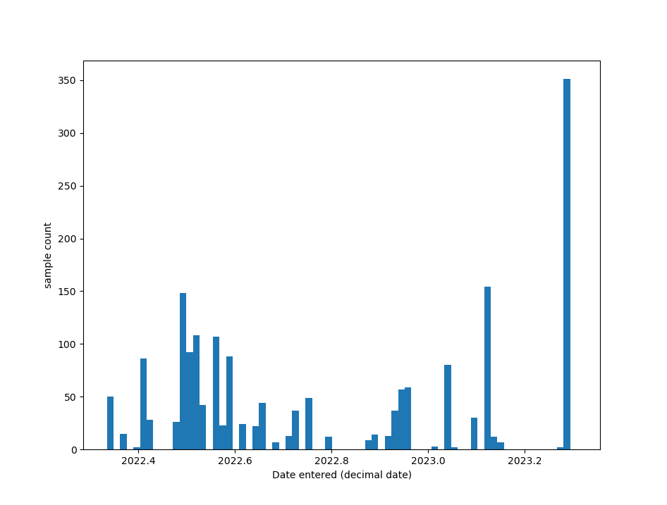
Onto the main event. Using a very simple python script, I was able to generate a histogram of all the samples added to ICE-D after March 11, 2022 and bin them approximately by 5 days. Data has been entered into ICE-D since Greg started the project in 2015, but March 11 of last year marked the date that we migrated the whole project into the new version. Thus, we lost the capability to determine exactly when data was entered prior to the migration. In the histogram, it is obvious that attendees to the Reston workshop shattered any 5-day data entry record in the last year since the migration. Greg and I spent a few hours in the afternoon of the first day teaching folks how to enter data, and they ran with it for the remainder of the workshop. In all, approximately 9 people entered over 350 samples into the database in about one full day’s worth of time! Excellent work, everyone. In my opinion, the histogram demonstrates two things:

1) The streamlined process for data entry into ICE-D now allows for rapid (and safer) uploading at a pace that might have been hard to match using the old method of data entry.

2) Perhaps more importantly, workshops work in engaging folks to contribute to ICE-D. I might be so bold as to say that folks at the Reston workshop actually had fun entering data. There were even suggestions of starting a data entry competition between this workshop and the next ones, but mentioning that now might be giving an unfair advantage to the next group of workshop attendees.

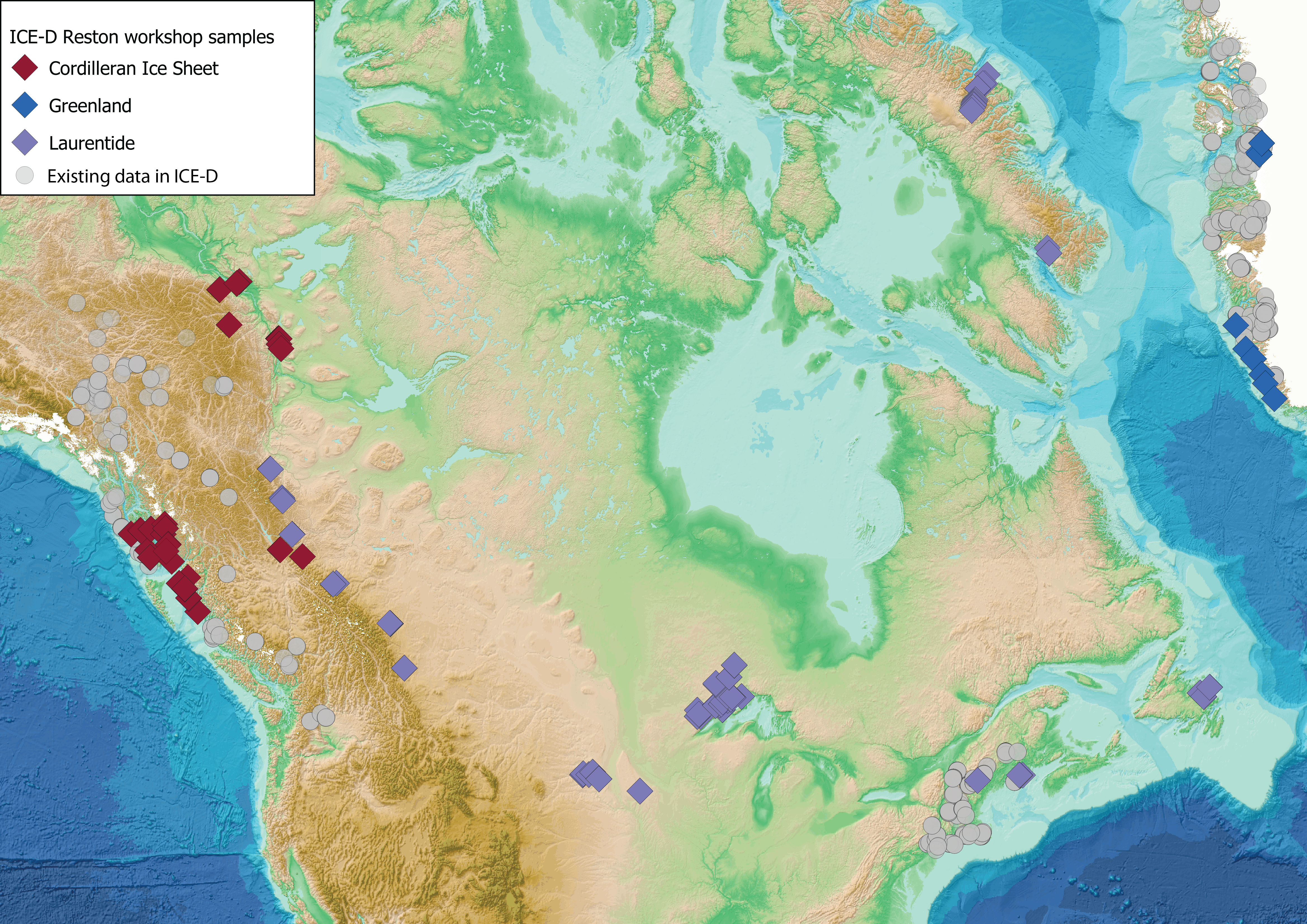
In general, the latest ICE-D workshop resulted in two new fully functional applications – the Cordilleran Ice Sheet and Laurentide Ice Sheet applications – that everyone can now explore on the ICE-D home page, seven new contributors to the ICE-D project (not including attendees who were already contributing), and approximately 350 new samples entered into the database. You can see the geographic distribution of the samples in the map figure below. Moreover, attendees learned how to easily pull data out of ICE-D using various platforms such python (see Fig. 1), QGIS/ArcGIS (see Fig. 2), and others for both data organization – no longer will attendees need to keep personal copies of cumbersome, error-laden excel spreadsheets – and visualizations/analyses.

I am thoroughly pleased and impressed with how the workshop went, and I am feeling optimistic about upcoming workshops. Furthermore, now that some folks are also learning useful skills for extracting data out of ICE-D, I can’t wait to see what fun and meaningful visualizations/analyses folks will come up with in the future. If you are interested in learning more yourself, we have several pages on the accompanying ICE-D wiki page. Here are some helpful links:

ICE-D wiki home page – https://wiki.ice-d.org/

ICE-D workshop program page – https://wiki.ice-d.org/workshops:start

ICE-D tutorials, visualization and analysis applications page – https://wiki.ice-d.org/applications:diy

We also now have a functioning listserv that we use to disseminate general ICE-D updates and news. The listserv additionally functions as an archive for general questions from ICE-D contributors and responses either from us or other ICE-D contributors. Please email me or Greg if you are interested in getting added to the listserv.

Happy big data era – Joe

Stickers!

Stickers are again available. Suitable for anyone interested or disinterested in subsurface production, although still slightly misleading for C-14.

Send a stamped, self-addressed envelope to:

Greg Balco, BGC, 2455 Ridge Road, Berkeley CA 94709 USA.

I will put some stickers in it and drop it back in the mail.

Find the gap! The late Holocene exposure-age gap in Antarctica, that is.

This is yet another post about using the ICE-D:ANTARCTICA database of exposure-age data from the Antarctic continent to learn something interesting about past changes in the Antarctic ice sheets. And it’s also another post focused on trying to digest the whole data set into a single figure. However, instead of focusing on what ice sheet changes are recorded in the exposure-age data set, it focuses on ice sheet changes that aren’t recorded. Yet. Specifically, hypothesize that in the process of shrinking from its Last Glacial Maximum size to its much smaller present size, the Antarctic ice sheet overshot and had to come back. Sometime in the last few thousand years, the ice sheet was smaller and thinner than it is now, and it’s recovered by growing back to its present configuration. From the exposure-dating perspective, the problem with this hypothesis is that you can’t prove that an ice sheet was thinner than present using evidence from above the present ice surface. So the point of this post is to think about how we might recognize an overshoot from exposure-age data anyway.

The idea of how to recognize a Holocene grounding-line overshoot is the subject of a paper in Cryosphere Discussions by Joanne Johnson, Ryan Venturelli, and a handful of other folks involved in Antarctic ice sheet change research, and the analysis described in this post was originally put together for that paper. Sadly, however, the paper is not entirely devoted to exposure-dating — exposure-dating gets only a meager few paragraphs buried in a fairly broad survey of geological and glaciological evidence — so this posting is a chance to explain the details of the exposure-dating application to the audience who will be disappointed that the paper couldn’t be about nothing but cosmogenic-nuclide geochronology.

For background, I will now spend four paragraphs on some context about the Holocene in Antarctica and why a Holocene grounding-line overshoot scenario is possible and/or interesting, before getting back to the exposure-dating details. If you already know about ice sheets or don’t care, skip forward four paragraphs. The background to this, then, is that the Antarctic ice sheets were the last of the Earth’s big ice sheets to shrink to their present size after the LGM. The much bigger Laurentide and Scandinavian ice sheets were completely gone, i.e., done shrinking to their present size of zero (or slightly more than zero if you count the Penny and Barnes ice caps as leftovers), about 7,000 years ago. They disappeared because they melted: the temperature in North America and Eurasia was too warm to sustain an ice sheet. In Antarctica, LGM-to-present ice sheet thinning was not because of melting — the temperature is still well below freezing always — but because of sea-level change. Water added to the oceans by melting of the big Northern Hemisphere ice sheets caused sea level to rise everywhere, including around Antarctica where glaciers flowing off the continent were calving icebergs into the ocean. Increasing water depth causes the iceberg calving rate to increase faster than the supply of ice from inland snowfall can keep up, so the glacier margin retreats inland until the water depth is shallow enough again that the calving rate can go back to a stable equilibrium. Thus, rising global sea level after the LGM eventually forced the Antarctic ice sheet to shrink, with a bit of a time lag: Northern Hemisphere deglaciation happened between about 19,000 and 7,000 years ago, but Antarctic ice sheet shrinkage really gets going about 15,000 years ago, and doesn’t stop until several thousand years after the Northern Hemisphere is done. In fact, most of the action in the LGM-to-present shrinking of Antarctica seems to have happened between about 8,000 and 4,000 years ago.

The reason this situation could cause an ice volume overshoot in Antarctica is that the sea level that the ice margin really cares about is not the average global sea level — which is just controlled by the amount of water that is or is not in ice sheets — but the relative sea level at the glacier margin. Because the Earth’s crust is somewhat elastic, when an ice sheet gets thinner, the land surface below springs up somewhat to compensate for the weight that is being removed, in the process of ‘glacioisostatic rebound.’ This process isn’t instantaneous, and it takes a few thousand years for the land surface to stabilize at its higher unloaded elevation. So, think about what is happening at the ice margin in Antarctica. Before 7,000 years ago, water is being added rapidly to the whole ocean, but the Antarctic ice sheet hasn’t thinned very much. Relative sea level change at this site is dominated by the global ocean getting deeper, and the ice margin perceives that sea level is going up. Sea level going up causes the glacier to retreat upstream and get thinner. After 7,000 years ago, on the other hand, the global ocean has stopped getting deeper, but the Antarctic ice sheet is thinning rapidly. This causes the land surface underneath the ice sheet to rebound. If the land surface is going up but the ocean isn’t getting deeper, the ice margin perceives that local relative sea level is now dropping. Decreasing sea level now forces glaciers to advance and get thicker.

So if we correctly understand what is happening here, the Antarctic ice sheet should have shrunk rapidly after the LGM as relative sea level rose. We know this happened. But it should have stopped shrinking some time after 7,000 years ago when relative sea level went from rising to falling, and then it should have expanded again. It should have been smaller and thinner at some point in the last few thousand years than it is now.

This is interesting because it’s not how we usually think of Earth history after the LGM: our conception of ice sheets on Earth is that they are the smallest now that they’ve been for a long time. However, that is probably oversimplified. It’s also likely that we are biased by the evidence for past ice sheet change that we happen to have available: it is easy to find evidence that an ice sheet was bigger in the past, because that evidence is not now covered by the ice sheet. Evidence that the ice sheet was smaller in the past is generally (although not always) inaccessible under the ice sheet. Fortunately, absence of evidence is not evidence of absence, so the rest of this posting will focus on using the exposure-age record to learn about where there is an absence of evidence that the ice sheet wasn’t smaller than it is now in the past few thousand years. Was it difficult to parse the quadruple negative in the last sentence? Read on for some help.

To boil down the long leadup here into something simpler, what we have is a lot of exposure-age data from above the present ice surface. What we want to know is whether the ice was thinner than it is now in the past few thousand years. Using data from above the ice, we can’t ever prove that the ice was thinner at a certain time. But we could prove that it wasn’t: if our hypothesis is that the ice was thinner than present 4,000 years ago, and we find some clasts above the present ice surface with exposure ages of 4,000 years, we have clearly disproved the hypothesis. It was thicker then, so it can’t have been thinner.

Look at some data that demonstrate this. Here is an exposure-age data set from a site in the central Transantarctic Mountains:

Exposure ages at this site appear to show a rapid ice surface lowering around 5,000 years ago, followed by slower, but continuous thinning between 5 ka and the present that culminates at the current ice surface elevation (shown by the blue dashed line). This data set doesn’t allow any time in the late Holocene during which the ice could have been thinner: there is pretty much a continuous age distribution of exposure ages above the present ice surface. The ice was thicker in the last few thousand years, so it couldn’t have been thinner.

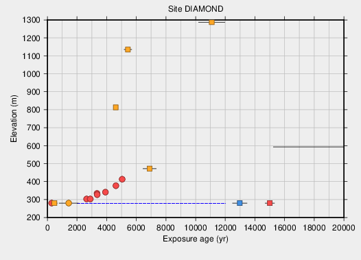
Here is another exposure-age data set, this one from the Hudson Mountains in the Amundsen Sea sector:

This is quite different. The ice surface elevation plummets from several hundred meters above present to the present surface in a short time between 6000 and 5500 years ago, and there is no evidence that ice was thicker than present between then and now. In other words, there is a late Holocene gap in the exposure ages. During this gap, the ice sheet could have been thinner. In fact, this seems likely because the alternative is that the ice thickness has been stable and unchanging for 5500 years: of course zero change is possible, but it seems unlikely in light of the fact that climate and relative sea level have been changing continuously during that time. But the point is that with this data set, we cannot disprove the overshoot hypothesis, that the ice sheet thinned in the last several thousand years and then thickened again to the condition that we see now.

To summarize all this and finally get to the point, exposure-age data sets from Antarctica, at least those with a decent number of data, should either allow a late Holocene overshoot, or not. We want to know what, if anything, we can learn about Antarctic ice sheet change using this reasoning. To investigate this, we will try to “find the gap” using the ICE-D:ANTARCTICA database and the following workflow:

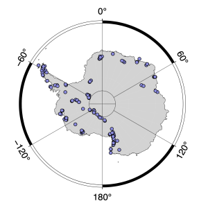
1. Find all sites where exposure ages in the Holocene (the last 12.5 ka) have been observed. There are 230 of these, shown by the small white circles in the next figure.
2. Reject sites with only a couple of Holocene exposure ages, or an array of a few ages that aren’t in stratigraphic order, leaving sites with more than approximately 5 data points that together form an age-elevation array in which exposure ages systematically increase with elevation.
3. Also discard coastal sites close to sea level where the lowest exposure ages are adjacent to ocean or a thin ice shelf, because where the ice thickness is zero now, it couldn’t have been thinner in the past.

These steps exclude a large number of sites with only 1 or 2 Holocene data, and a handful that are at sea level, leaving 28 sites or groups of closely spaced sites that show an extensive enough Holocene age-elevation array that one can make a reasonable decision about whether or not there is a late Holocene gap. Now,

4. Plot these 28 sites on a map and figure out which is which.

The result is this:

This is another cool image that encapsulates a lot of information about Antarctic ice sheet change in one place. In fact, it is pretty dense. You should be able to enlarge it by clicking. What is going on here is as follows. First, exposure age and sample height above the present ice surface for the 28 exposure-age data sets that came out of the screening process are plotted around the edges. Numbers and color-coding (redundantly) index each data set to its location in Antarctica. Then, sites where there is a late Holocene gap are plotted as squares (and have a gray background in the age-elevation axes). Those where there is no space for a gap are plotted as circles (and have white backgrounds).

The first thing that is important about this plot is that there are both kinds of data sets. There are sites that clearly show a gap, and sites that clearly don’t have space for a gap. Surprisingly, there are relatively few sites that are ambiguous: nearly all sites either have an age-elevation array that intersects (0,0) — leaving no gap — or that obviously hit the x-axis in the middle Holocene. There are only a couple of examples where it’s hard to tell (for example, 13 is a little vague).

The second thing that is really interesting about this plot — and that I did not expect to see — is that the two types of sites are geographically patterned. The gap is ubiquitous in the Amundsen Sea (10-12), in the Weddell embayment (13-18), and in the outer Ross Sea (20-22). However, there are nearly zero gaps in any part of Antarctica that flows into the Ross Ice Shelf (1-9, 26-28). In East Antarctica, there’s only one site that got through the screening (19), so it’s hard to say much about the East Antarctic margin. But for the rest of Antarctica, leaving aside the northern Ross Sea sites that mostly pertain to large alpine glaciers flowing out of Victoria Land instead of the ice sheet as a whole, it is clear that there is a gap that permits a late Holocene overshoot in the Amundsen and Weddell sectors of the ice sheet, but not in the Ross sector.

Does this make sense? Well, there is some independent evidence of a Holocene overshoot-and-recovery cycle in the Weddell embayment. So that is consistent with the distribution of exposure-age gaps. So far, there is not much evidence either way in the Amundsen Sea region. Unfortunately, there is also some evidence for an overshoot in the Ross Sea, which is not what the exposure-age data say. Overall, however, what this shows is that what we think ought to have happened from first principles — ice thinning in the last few thousand years followed by thickening to the present configuration, driven by relative sea-level change — is, in fact, not contradicted by the exposure-age data set for most of Antarctica. In fact, the exposure-age data rather favor it.

Except around the Ross Ice Shelf. Figure that out, readers.

Impossible as it seems, the cosmogenic-nuclide job market looks like the job market in the rest of the US

Cosmogenic-nuclide geochemistry is not generally noted for being anything like real life. It can’t even be explained to most folks without a 20-minute briefing on nuclear physics, and it is rare to find any normal person off the street who is even willing to get through the entire 20 minutes. The business model for the field involves taking bright undergraduates with many skills and great potential for success…and using the lure of exotic fieldwork in places like Antarctica and Greenland to systematically divert them into successively more arcane graduate programs, eventually leading to an unlikely chance of employment in a vanishingly small number of poorly-salaried positions. This is precisely the opposite of the economic model for prominent fields otherwise suitable for bright undergraduates, such as law, medicine, and finance, in which enduring an arduous training program yields guaranteed employment at a high salary. This may only prove that cosmogenic-nuclide geochemists are just people who failed the marshmallow test, but for present purposes highlights the deep divide between this field and the rest of the global economy. We are fishing in different oceans.

The purpose of this blog posting, therefore, is to highlight an unusual convergence between the two. The big economic story right now as the US emerges from the COVID-19 pandemic is that it is almost impossible to hire workers. Depending on who you are, this is either (i) Joe Biden’s fault for rewarding slackers with rich unemployment benefits, or (ii) a welcome rebalancing of the relationship beween capital and labor. What is bizarre is that this also appears to be a problem in the alternative economy of cosmogenic-nuclide geochemists. Recently, the U.S. National Science Foundation provided some funding to support the ICE-D database project, which has been the subject of quite a number of blog entries in recent years and, basically, is supposed to be producing a so-called transparent-middle-layer database to facilitate regional- and global-scale research using cosmogenic-nuclide data. Part of this funding is for postdoctoral support, and since late May we have been advertising for this position. Sure, maybe the ICE-D website itself is not the greatest way to reach a broad audience, but it’s also been posted with AGU, and the Twitter announcement got 8000 views, which isn’t huge by global Twitter standards, but is probably well in excess of the total number of geochemists in the US.

However, so far this advertisement has only generated ONE APPLICATION that passed an initial screening for qualifications in some reasonably related field. One is an extremely small number for even a postdoc position in a fairly obscure field, and it’s not enough to conclude that we have made a reasonable effort to attract a representative pool of applicants, so we are continuing to advertise. But this is very strange. From the perspective of the rest of the US economy, we might expect it to be hard to fill this position. But this is the cosmogenic-nuclide geochemistry economy! It should have no relation. So, why is this? I can think of a few possibilities.

One: cosmogenic-nuclide geochemists are kicking back and collecting unemployment. Frankly, this seems unlikely, and we did make sure to set the salary above the total of California unemployment and the Federal supplement. But if this is the problem, it’ll be fixed in a couple of months when the supplement expires.

Two: everyone has a job already. This seems very possible, as NSF has been aggressively giving out supplemental funding to extend existing PhD and postdoctoral salaries so as to bridge over the disruption to nearly all field and lab work during the 2020-21 academic year. In addition, I haven’t attempted to look at this systematically, but my impression is that a large number of postdoc positions have been advertised recently on Earth science newsgroups. These together would imply a pipeline stoppage in which all postdocs have jobs, but no PhD students will need to become postdocs until next year. If this is the explanation, we might expect to have to wait 6 months or so before seeing a decent number of applications. Not ideal.

Three: international travel is still closed. This position is open to non-US citizens, and under normal circumstances I would expect to see a lot of international applications. Let’s face it, places outside the US, in particular Europe and the UK, have produced a lot more early-career cosmogenic-nuclide geochemists than the US in recent years. However, right now it is extremely unclear whether or not, and under what conditions, a European Ph.D. would be able to enter the US right now to actually take the job. I don’t know the answer to this myself, but I agree it doesn’t look great in the near term. Solving this problem, again, might take 6 months to a year.

Four: there are structural obstacles to folks moving right now. Mainly, “structural obstacles” in this context means “I have kids and there is no school or child care right now.” Just considering the demographics, this doesn’t seem super likely, but it could be a show-stopper for individuals. By the way, if this describes you, this might be fixable. Contact me.

Five: Berkeley is impossibly expensive. Berkeley is in the heart of one of the most expensive metropolitan areas in the world. Although BGC aims to have postdoctoral salaries be equivalent to those specified by NSF in their postdoctoral programs (currently $64k), these are set nationally and are low compared to the cost of living here. This is a serious problem and I don’t have a good way to fix it, except to move somewhere else myself, which may be the only long-term solution but is tough to implement immediately. However, if you would have applied for this job if not for the cost-of-living situation, please contact me and let me know. If we are going to figure out some way to raise salaries, it’ll be because of emails that say “I am a great scientist but I can’t work at BGC because Berkeley is too expensive.”

Six: the software part of the job description is off-putting. I’ll give this one some attention because I’m a bit worried about this: I know of several candidates who would be qualified for this job and have applied for other recent postdocs related to cosmogenic-nuclide geochemistry, but have not applied for this one, and I don’t know why. Also, this is one of the possibilities that I can do something about fixing. Basically, the point of the ICE-D project is to build computational infrastructure to make it possible to look at large data sets of cosmogenic-nuclide data to do things like paleoclimate analysis, slip reconstructions on complex fault systems, ice sheet model validation, etc. Doing this requires some knowledge of both cosmogenic-nuclide geochemistry and software development. People who are good at both of these things are rare, of course, but the job description for this position includes both. It’s asking for someone who (i) at least cares about cosmogenic-nuclide geochemistry and how it’s applied to important Earth science problems, and also (ii) is at least interested in software design. It may be that the job description has too much of (ii) in it, and otherwise qualified cosmogenic-nuclide geochemists are suffering from impostor syndrome about the software part.

Unlike US immigration policy and apartment rents in Berkeley, this one is fixable. I’ll start by admitting how many programming classes I’ve ever taken, which is zero. Whoever you are, you have probably had more training in this than I have. I am a terrible impostor when it comes to software.

The next point is that software development is not that hard. The most important thing from the perspective of this project is having an idea about what you want to do with large amounts of cosmogenic-nuclide data, and a willingness to learn what you need to learn to implement this idea. Once you have this, it is not that hard to learn enough to implement what you want to do in ways like we have already set up with the ICE-D project. Also, there are actual professional software developers involved with this project. You don’t have to do it yourself. In other words, we don’t expect to find a candidate for this who already knows a lot about cosmogenic-nuclide geochemistry AND software development. This would be very unlikely. What we want is a candidate who would like to become this person in future.

Finally, to get back to the point of the beginning of this blog entry, the really unusual aspect of this postdoctoral position, which seems kind of attractive to me, is that it’s a fairly rare opportunity to break out of the death spiral of scientific overspecialization. The problem that this project is aiming to fix — how to do something with lots of data that together are too complicated for an Excel spreadsheet — is, uh, not exactly unique to geochronology. If you spend a couple of years working on this, no one is going to tell you you can’t describe yourself as a ‘data scientist’ in future job applications, which is likely to lead to many options that are not generally open to ‘cosmogenic-nuclide geochemist.’ So far, one postdoc has worked on the ICE-D project. They left early to work as a data scientist for a cybersecurity startup. If you still want to be a professor at a small college regardless, can it hurt to be able to teach “data science” as well? Possibly not.

To summarize: if you are reading this and you considered applying for this job but didn’t do so for one of the reasons listed above, or some other reason, please contact me and let me know why. That would be extremely helpful and could make it possible to fix the problem. If you didn’t know about it before, take a look at the description and circulate it. Thanks much.

Antarctic deglaciation in one figure

This post is not so much about how one generates cosmogenic-nuclide exposure-age data, but what one does with it. Especially when you have a lot of it. The example focuses on exposure-age data from Antarctica that record the LGM-to-present shrinkage of the Antarctic ice sheets.

First, the background. Right from the beginning of exposure-dating, one of its most useful applications has been figuring out what happened to the Antarctic ice sheets. Even though only a tiny amount of Antarctica is actually ice-free at the moment, the areas that are ice-free are thoroughly stocked with glacial deposits that were deposited when the ice sheet was thicker or more extensive. Unfortunately, it is really hard to date these deposits, because they are just piles of rock, with almost nothing organic that can be radiocarbon-dated. Enter exposure dating. Cosmogenic-nuclide exposure dating is nearly perfect for Antarctic glacial deposits, because most of the time the rock debris in these deposits is generated by subglacial erosion of fresh rock that hasn’t been exposed to the cosmic-ray flux, so when it gets deposited at a retreating ice margin, its subsequent nuclide concentration is directly proportional to how long it has been exposed. Let’s say you visit a peak sticking out of the ice that looks like this:

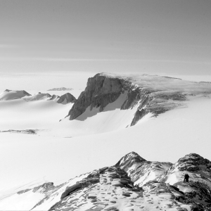
This is a place called Mt. Darling, in Marie Byrd Land in West Antarctica. Upon the glacially-scoured bedrock of this summit you find things that look like this:

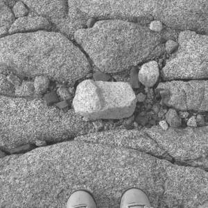These are “erratic” clasts that don’t match the bedrock, so must have been transported by somewhere else when the ice sheet was thicker, and deposited here by ice thinning. If you measure the exposure age of a bunch of erratics at different elevations, you get this:

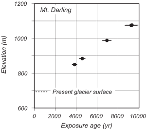Exposure ages are older at higher elevations and younger at lower elevations, indicating that this peak has been gradually exposed by a thinning ice sheet during LGM-to-present deglaciation between, in this case, 10,000 years ago and the present. This is a classic application of exposure dating, first implemented in West Antarctica circa 2000 in a couple of studies by Robert Ackert and John Stone (this example is from the Stone study).

The usefulness of this technique in measuring how fast the Antarctic ice sheets shrank after the LGM, and therefore in figuring out the Antarctic contribution to global sea level change in the past 25,000 years, immediately inspired everyone else working in Antarctica to get busy and generate more of this sort of data. Now, 20 years later, we have a lot of it. Usefully, these data are all compiled in one place in the ICE-D:ANTARCTICA database.  At the moment, there are 163 sites in the database at which some LGM-to-present (that is, 0 to 25,000 years before present) exposure-age data exist, and they are all over Antarctica, at least in all the areas where there is some rock outcrop available:

So, the challenge for this blog posting is to use these data to generate some kind of overall picture that shows the overall response of the Antarctic ice sheet to LGM-to-present deglaciation. And the further challenge is to do it with an automated algorithm. It is way too much work to individually curate 163 data sets, and if it is written as a script then it can be repeatedly run in future to assimilate new data. The main problem that the hypothetical no-humans-involved algorithm needs to deal with is that the data sets from most of the 163 sites are much messier than the example from Mt. Darling shown above. For that example, you just draw a line through all the data and you have the thinning history at that site during the period represented by the data. Done. However, consider this site:

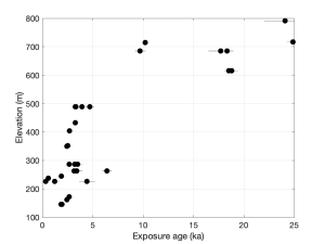
These data are from a place called Mt. Rea, also in Marie Byrd Land. At some elevations, there is not just one exposure age, but a range of exposure ages. The reason for this is that a lot of these samples were not deposited during the LGM-to-present, most recent deglaciation. They were deposited in some previous interglaciation prior to the LGM, exposed for a while, covered by LGM ice but not disturbed, and then exposed again. Thus, their exposure ages are older than the age of the most recent deglaciation. This problem is very common in Antarctica because the thicker LGM ice sheet was commonly frozen-based, so did not erode or remove pre-existing glacial deposits.

The usual means of dealing with this is to assume that the population of exposure-dated samples at a site consists of some mixture of (i) samples that have only been exposed since the most recent deglaciation, and (ii) samples that were exposed in prior interglaciations and covered at the LGM. We want to consider (i) and ignore (ii). This assumption implies that the youngest sample at any particular elevation should give the correct age of the most recent deglaciation, and other samples at that elevation must overestimate the age. In addition, the basic geometry of the situation — that ice cannot uncover a lower elevation until and unless it has already uncovered all higher elevations — leads to the basic concept that the true deglaciation history inferred from a data set like this one is the series of line segments with positive slope (that is, increasing age with increasing elevation) that most closely bounds the left-hand (i.e., younger) side of the data set. It is fairly straightforward to turn these rules into a MATLAB function that will generate an allowable deglaciation history for a typical set of messy exposure-age data from some site. Here is the result for this data set:

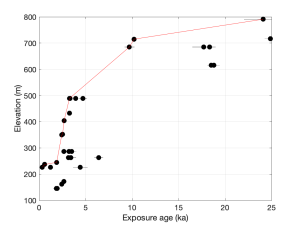
This algorithm is extremely simple, but most of the time comes up with about the same interpretation that a knowledgeable human would, although it has a tendency to take outliers on the young side slightly more seriously than the human. So, let’s apply this to all 163 data sets. Of course, it is only possible to apply this algorithm to a data set that contains at least two samples for which the higher sample is older, so this step excludes 64 sites with either single measurements or small numbers of data that can’t be fit with a positive slope, leaving 99 sites. Here are the results: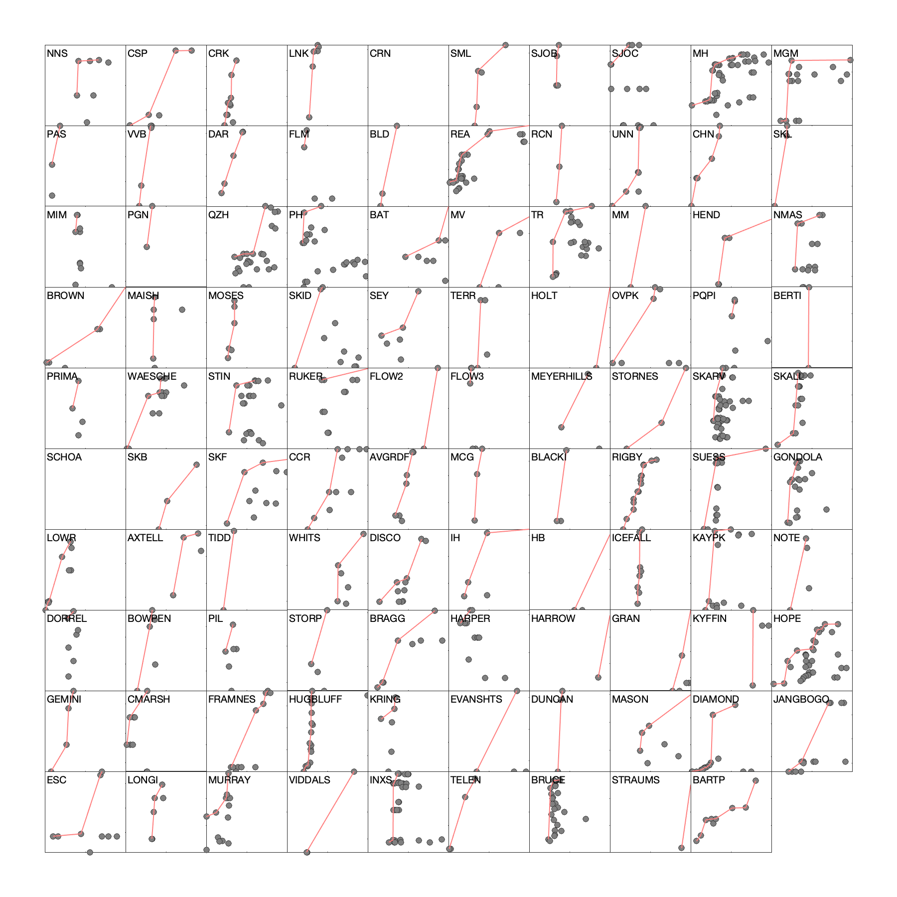In each of the panels in this plot, the x-axis is exposure age from 0 to 25,000 years. The y-axis is always elevation, but the limits vary with the elevation range of the data set. The dots are the measured exposure ages, and the red line is what the pruning algorithm comes up with. Readers who actually know something about the details of some of these sites may notice that this algorithm is not quite doing exactly what they would do — the main difference is that it is ignoring information from some papers to the effect that samples at the same elevation at a particular site may not reflect the same amount of ice thickening. But what we see here is that the majority of LGM-to-present data exposure-age data sets from Antarctica do, in fact, indicate LGM-to-present thinning of the ice sheet.

The next step is to put all these deglaciation histories on the same page:

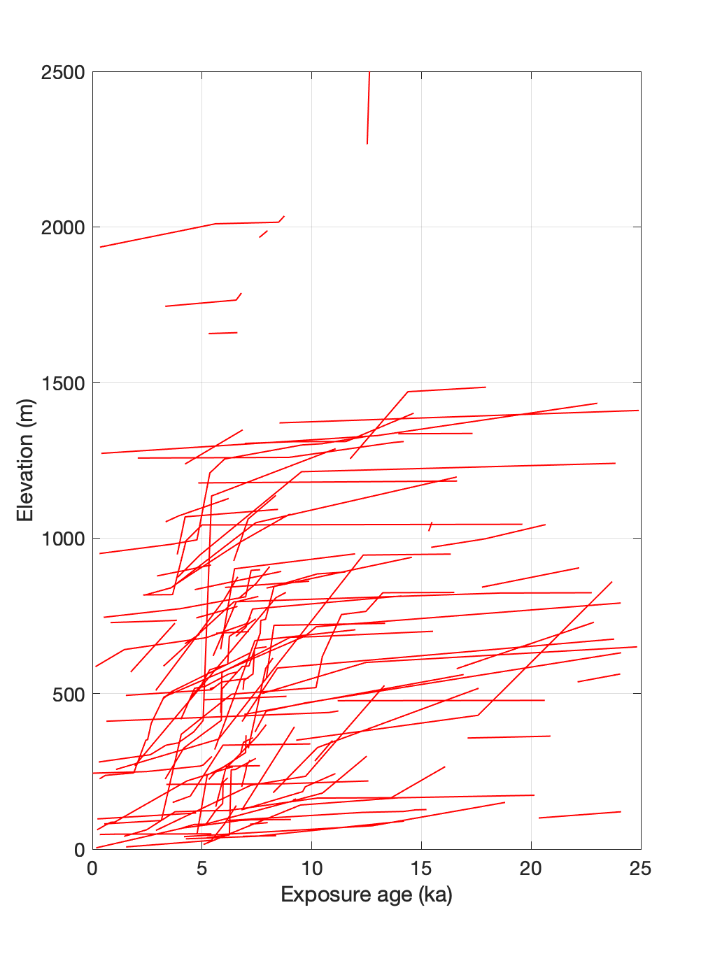
In this plot they are shown with actual elevations. This plot gets us pretty close to the goal of representing all the exposure-age data pertaining to Antarctic deglaciation on a single figure, and it is interesting. What is most interesting is that it shows very clearly that rapid ice sheet thinning is very common in the middle Holocene, between about 4-8 ka, and very rare otherwise. This is not necessarily expected. It’s also neat because it highlights the fact that when you have a large enough amount of data, even if you think that either the data from some sites are garbage or the pruning algorithm is delivering garbage results sometimes (both of which are probably true), it is not necessary to rely on any one particular record to have high confidence in the overall conclusion that rapid thinning is much more common in the mid-Holocene than at any other time. If we wanted to strictly disprove the hypothesis that a couple of sites experienced rapid thinning at younger or older times, then we would have to think in more detail about the details of the few anomalous sites. And it is possible that the pruning algorithm is biased slightly young by accepting a few young outliers that humans might have rejected. But I will argue that the broad conclusion from these data that nearly all recorded rapid thinning events took place in the mid-Holocene is very error-tolerant. It has low dependence on the pruning algorithm performance or on any one or a few individual sites.

Another thing that is interesting about this plot is that the period during which rapid thinning took place is basically the same at all elevations. Ice sheet thinning forced by grounding line retreat, for example, should be evident first at low-elevation sites near the grounding line and then later at higher-elevation inland sites. There is no evidence of that in this plot. Everything seems to basically go off at once.

Another way to show this is to move these results from time-elevation space to time-thinning rate space, as follows:

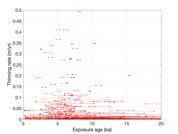
What happened here is that, remember, each deglaciation history generated by the pruning algorithm is a series of line segments. This plot just shows the time extent of each line segment plotted against its slope, which is the deglaciation rate in meters per year. For example, suppose a thinning history has a line segment whose endpoints are 100 m elevation at 5 ka and 200 m elevation at 6 ka. 100 m of elevation change in 1000 years is 0.1 m/yr, so in the second plot this would be represented as a line that extends from x = 5 ka to x = 6 ka, and has a y-coordinate of 0.1 m/yr. This plot has several weird pathologies, mostly focused on the fact that because of the basic properties of averaging, only short line segments can have steep slopes…the longer the period of averaging, which is just determined by what data were collected, the lower the slope is likely to be. However, it is very effective at highlighting the basic  thing that we learn from these data, which is that nearly all rapid ice sheet thinning events in Antarctica during the LGM-to-present deglaciation took place during a relatively short period between about 4 and 8 ka. Even if you ignore the extremely high thinning rates shown by a handful of short lines, the cloud of longer lines near the bottom of the plot shows the same effect. Thinning rates were relatively slow basically everywhere until well into the Holocene, and all the action happens in a few thousand years in the middle Holocene.

Although of course rapid mid-Holocene thinning has been observed and discussed at length in a lot of studies focusing on one or a few of the data sets that are summarized here, it is not very clear from first principles why this should be true. Because nearly all Antarctic glaciers are marine-terminating, the simplest glaciological explanation for accelerated ice sheet thinning in Antarctica has to do with nonlinear grounding line retreat. Sea level rise or ice thinning results in the grounding line of a marine-based part of the ice sheet becoming ungrounded, which triggers rapid thinning and retreat until the grounding line can stabilize again at some upstream position. This process should be driven by global sea level rise associated with melting of the Northern Hemisphere ice sheets. However, global sea level rise starts about 19,000 years ago, is fastest 14-15 ka, and is basically complete by 7-8 ka. It appears that nearly all of the Antarctic outlet glaciers that we have exposure-age data for waited until sea level rise was almost over before responding to sea level rise. Weird.

The basic concept that probably resolves most of this apparent discrepancy, as mostly inferred from ice cores and implemented in ice sheet models of the last deglaciation, probably has to do with the fact that climate warming after the LGM greatly increased accumulation rates throughout Antarctica, This seems to have somewhat balanced the tendency toward grounding line retreat and sustained a relatively large ice sheet until the mid-Holocene. And in addition, there are important biases in the exposure age data set, specifically that many of the sites where we have exposure-age data were completely covered during the LGM, so they can only preserve a record of deglaciation for the time period after they first became exposed. But even so, sites that were not covered during the LGM show slow thinning until well into the Holocene. And nearly all ice sheet models have a very strong tendency to initiate rapid thinning around the beginning of the Holocene, which is still a couple to a few thousand years before it is recorded by exposure-age data.

Regardless, this is a decent attempt at the goal of showing nearly all of the exposure-age data set that is relevant to LGM-to-present deglaciation in one figure. It highlights that even if you have a lot of messy data sets, considering them all together leads to what I think is a fairly error-tolerant conclusion, that doesn’t critically depend on any of the data sets or assumptions individually, that most of the action in Antarctica during the last deglaciation took place during a short period in the middle Holocene.

An end to the Cl-36 monopoly

For the last several years, folks interested in computing exposure ages from beryllium-10 or aluminum-26 measurements have enjoyed a proliferation of online exposure age calculators enabling them to do this. This seems like a good thing, because it’s useful to be able to make sure that whatever conclusion you are trying to come to doesn’t depend on the specific calculation method you chose — it should be true for any reasonably legit method and choice of parameters — and, in addition, competition keeps prices down. In fact, this works so well that all the online exposure age calculators are free.

On the other hand, folks interested in chlorine-36 exposure dating have, alas, not enjoyed the same diversity of choices. So far, the only option for Cl-36 exposure-dating has been the ‘CRONUSCalc‘ service, which works great but has several practical disadvantages for some users. For one, it has a fixed production rate calibration and no means of experimenting with alternative calibrations, which could be either a feature or a bug depending on your attitude. Second, it was designed for precision and not speed, and it is quite slow, returning results asynchronously via email instead of immediately via the web browser. And, personally, I find the input format maddening because all the measurements are at the beginning and all the uncertainties are at the end. This is weird. Of course, none of these issues are catastrophic, show-stopping, or really even more than mildly annoying, but, more importantly, if there is only one option for calculating Cl-36 exposure ages, it is hard to tell how sensitive your conclusions are to whatever assumptions the CRONUSCalc developers made in putting together the rather complex Cl-36 code. And also, monopolies are financially precarious for customers. What if CRONUSCalc suddenly requested your credit card info? You would have to pay up. No choice. Not good. 

So, the purpose of this post is to describe progress in ending the Cl-36 monopoly. First, the group responsible for CREp has focused on the calibration issue, and is working on a Cl-36 adaptation of CREp that, like the existing version for Be-10 and Al-26, will have several calibration options. This is not done yet but I am reliably informed that it is fairly close. Second, I finally finished a draft version of a Cl-36 exposure age calculator that, like the existing version 3 of the online exposure age calculators, is designed to be much faster than CRONUSCalc so that it can serve as a back end for dynamic exposure age calculations used by the ICE-D online databases. The point of this blog entry is to briefly explain what is in it and, less briefly, discuss the messy subject of production rate calibration for Cl-36.

The overall summary is that now there are two choices. You can wait until the end to decide whether they are good choices, but they are choices. 

So, the problem with Cl-36 exposure age calculations is that there are too many ways to produce cosmogenic Cl-36. In most commonly used nuclide-mineral systems, e.g., Be-10, Al-26, He-3, C-14, and Ne-21, nearly all production is by spallation on one or two target nuclei, with a small amount of production by muons. For exposure-dating, you need to do some kind of a muon calculation, but it doesn’t have to be very precise because it only accounts for a few percent of surface production. So, in general, you are just scaling a single production reaction on one or two elemental targets. Mostly these nuclides are measured in quartz, so the target chemistry isn’t even variable. That is pretty straightforward. Cl-36, on the other hand, is produced by (i) spallation on four different target nuclei (K, Ca, Fe, Ti) whose concentrations are quite variable in rocks and minerals commonly used for Cl-36 measurements, (ii) muons, and (iii) thermal neutron capture on Cl, which is, basically, a mess, and requires a calculation of the entire thermal and epithermal neutron field surrounding the sample. Thus, the first problem in extending the existing online exposure age calculator to Cl-36 is that we have to compute production due to four different spallation reactions, which all have slightly different scaling, instead of one, and also add an algorithm to calculate production rates via the thermal neutron pathway. Muons are basically the same as before, with the exception that you have to account for variable target composition in computing Cl-36 yields from muon reactions. However, this is all feasible, and for this application I have just implemented the thermal neutron and muon calculations from an extremely clear 2009 paper by Vasily Alfimov. So that is done, although there are a few minor issues left having to do with calibration of muon reaction yields from K and Ca. 

The real problem that arises from the diversity of pathways for Cl-36 production is not that it is hard to code — that is a pain but is manageable. The problem is that it is hard to calibrate. For Be-10 in quartz, for example, it is straightforward to find a lot of different calibration sites where the same reaction — high-energy neutron spallation on Si and O — is happening in the same mineral. Thus, you are fitting a scaling algorithm to data that are geographically variable, but are always the result of the same reaction. You can apply a large data set of equivalent measurements to evaluate reproducibility and scatter around scaling model predictions. For Cl-36, on the other hand, target rocks or minerals for Cl-36 measurements at different calibration sites not only have different ages and locations, they have different chemical composition, so not only is the production rate from each pathway geographically variable in a slightly different way, the relative contribution of each pathway is variable between samples. 

The result of this is a bit of a mess. Results from two sites are not comparable without applying transformations not only for geographic scaling but also for compositional variability. Of course, increasing complexity brings not only increased messiness but also increased opportunities for complex methods to reason your way out of the mess, and anyone who has ever had a class in linear algebra will immediately grasp that the problem is, in principle, solvable by (i) collecting a lot of calibration data with the widest possible diversity of chemical composition and production mechanisms, and (ii) solving a large system of equations to get calibration parameters for the five production rates. In fact, that would be really cool. If you have no idea what I am talking about, however, that’s OK, because the application of this approach to large sets of Cl-36 calibration data by different research groups, mostly in the 1990’s and 2000’s, yielded thoroughly inconsistent and largely incomprehensible results. Theoretically, two applications of this idea to different calibration data sets should at least yield the same reference production rate for at least some of the pathways, but in reality different attempts to do this yielded estimates of the major production parameters (e.g., the reference production rate for spallation on K or Ca) that differed by almost a factor of two. That is, even though two calibration attempts might yield a good fit to large data sets consisting of samples with mixed production pathways, if you want to use those results to compute an exposure age from a sample with only one of those pathways, your exposure ages will differ by a factor of two. Figuring out why is extremely difficult, because this calibration approach yields parameter estimates that are highly correlated with each other, such that a mis-estimate of, say, the production rate from K spallation might actually arise from a mistake in handling production from Cl. Essentially, although this approach is mathematically very attractive and should work, so far history has shown that it does not work very well. 

The alternative approach to production rate calibration is to cast aside the samples with multiple production pathways and focus on collecting a series of calibration data sets, each consisting of samples where Cl-36 production is dominated by one pathway. For example, Cl-36 production in K-feldspar separates with low native Cl concentrations is nearly all by K spallation, and likewise production in plagioclase separates is nearly all by Ca spallation. This approach was mostly first used in a series of papers dating back to the 1990’s by John Stone, and was also what was adopted for production rate calibration for the CRONUSCalc code. Although it is mathematically much more boring and has the significant disadvantage that the need to obtain calibration samples with very specific chemistry greatly reduces the size of each calibration data set and therefore makes it hard to quantify fit to scaling models, it has the advantage that it actually works. The calibration of each pathway is independent of the others, so it is not necessary to, e.g., have a complete understanding of thermal neutron production to date samples where production is mostly by K spallation. 

I am using this approach. The pathway-specific calibration data sets used for CRONUSCalc, however, were very small, so I am using larger sets of literature calibration data from more sites to try to reduce the dependence on any one site. Of course, because the whole point of the version 3 online exposure age calculators is to be part of the overall ICE-D database ecosystem, the entire development project is somewhat elaborate and  looks something like this:

1. Figure out an extended input format for Cl-36 data that looks like the existing He-Be-C-Ne-Al input format and includes major and trace element compositions (and doesn’t drive me nuts like the CRONUSCalc input format). That’s here. 
2. Finish the Cl-36 online exposure age calculator part. Done, mostly. 
3. Incorporate Cl-36 calibration data in the ICE-D:CALIBRATION database of production rate calibration data. Fix up the web server to display the data in the format from (1) above. Done, and now this page provides access to the pathway-specific calibration data sets used for CRONUSCalc and also the expanded ones that I am using. There are still a lot of Cl-36 calibration data not yet entered, but there are enough to get started. 
4. Modify the other ICE-D databases to include Cl-36 data, spit it out in the appropriate format for online exposure age calculator input, and compute Cl-36 exposure ages.  That’s done for ICE-D:ALPINE (here is an example), but not the others. 
5. Do the production rate calibration well enough that the exposure ages aren’t obviously wrong. 

Those parts of the project are more or less complete, and here are the results of the calibration in (5), for St and LSDn scaling. As in other literature having to do with production rate calibration, the procedure for making these plots is to (i) fit the various production parameters to the calibration data, (ii) use the fitted parameters to compute the exposure ages of the calibration data, and then (iii) compare those to the true ages of the sites. We’d like to see the differences from unity to be about the same scale as the individual uncertainties, and also not systematically correlated with scaling parameters like latitude and elevation. 

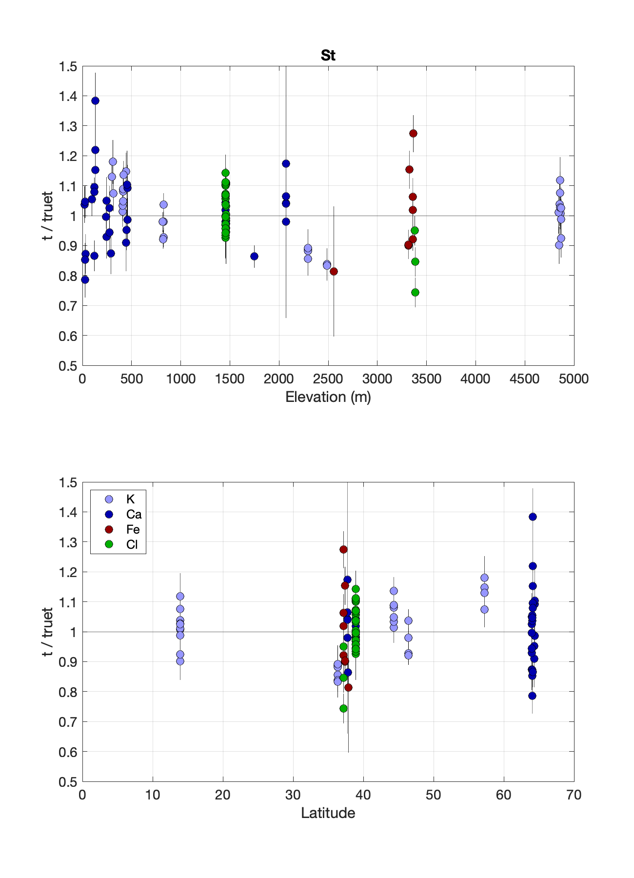
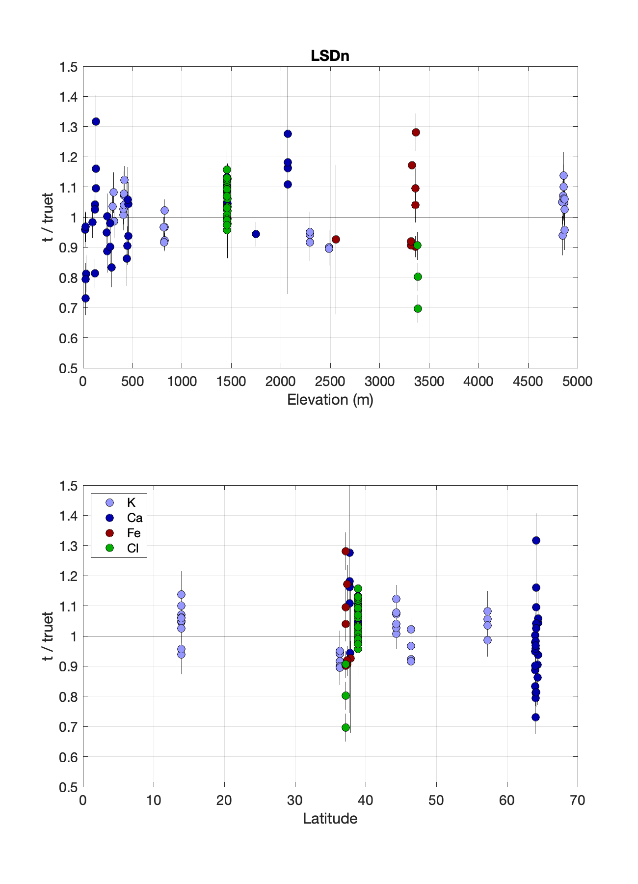
The data are color-coded by dominant production pathway, and the calibration data sets used are this one for K, this one for Ca, this for Fe, and this for neutron capture on Cl. Of course these are moving targets so they might be different by the time you read this. As Cl-36 calibration results go, these are not bad. Scatter for K-spallation data is only 7%, comparable to fitting scatter for Be-10 and Al-26. It’s larger (10%) for Cl-dominated production, which is not surprising — the only reason it is that good is that the Cl-dominated data set is small so far —  but it is also much larger (13%) for Ca-spallation data, which is more surprising. It looks like maybe some work on Ca-spallation calibration data is needed. But even though this is not a huge calibration data set, I think this result is good enough to make calculated exposure ages believable, and even reasonably accurate for simple target minerals like K-feldspar. 

So that’s good. It basically works. Now you have a choice of two options, at least until the CREp version is finished. Also, progress can happen on including Cl-36 data in the ICE-D databases. However, there are still a few things that are not done:

1. There are a couple of small things relating to muon production  that need to be fixed up. These are not very important for surface exposure age calculations. 
2. A couple of minor decisions on how to handle arcane aspects of input data still need to be made. Like, if there is an LOI value included as part of an XRF analysis, do you assume that is water? CaCO3? Ignore it? No idea. 
3. It is generally not obvious how to compute uncertainties for Cl-36 exposure ages. The approach at present uses estimates of scaling uncertainty for each production pathway and the same linearization as is used in the existing exposure age calculators, but there seems to be an undiagnosed bug that causes it to break for some target chemistries. Needs a bit of work. 
4. More calibration data from existing literature could be added. 
5. It could be faster. It’s fast enough that it doesn’t take too long for the ICE-D web pages to load, but it’s slower than the He-Be-C-Ne-Al version. This might just be because of the plotting overhead for the production-proportion plots, but it could be improved a bit. 
6. Of course, there is not really any documentation. 
7. Multiple nuclide plots. Cl-36/Be-10, Cl-36/Ne-21, etc. Really interesting. Possible to implement and potentially rather useful, but the banana is shaped differently for every Cl-36 production pathway, and figuring out how to get all that into one figure is kind of daunting. 
8. Production rate calibration. The current He-Be-C-Ne-Al online exposure age calculators have a production rate calibration interface that allows you to enter arbitrary calibration data for one nuclide, fit the scaling methods to those data, and then proceed to compute exposure ages in an internally consistent way. It is going to be hard to replicate this for Cl-36, mainly because if one is allowed to enter completely arbitrary Cl-36 calibration data, many data sets that one could enter simply would not work. For example, if the input data were dominated by K production and you used the resulting calibration to compute exposure ages for Ca-dominated samples, you would probably get the right answer only by accident. It is possible to envision a method by which you could enter calibration data for one pathway at a time and use default values for the others — this would address quite a lot of useful applications while making it a little harder to screw up completely — but this approach would also require quite a lot of error checking to make sure the calibration data set had the advertised properties, and the unknown-age samples had similar production pathways to the calibration data. In any case, I am not sure what the most sensible way to do this is. 

 

 

 

 

Version 3 erosion rate calculator benchmarked, finally

This is another post about the very slow upgrade of the online exposure age and erosion rate calculators to the latest version 3. As alluded to in the previous post, erosion rate calculations somehow always seem like a lower priority, and that part of the upgrade was a bit delayed. However, the version 3 erosion rate calculator is now more or less complete (although a couple of interesting bugs having to do with very high erosion rates survived until a couple of weeks ago and have just now been fixed), and seems to be mostly in use.

However, one problem with the version 3 erosion rate calculator that hasn’t really been addressed is that even though I personally think it probably mostly works, no one really has any idea if this is true. For one thing, the documentation is not particularly good and could be improved, and for another, at least as far as I know, there hasn’t been any systematic testing against either the previous version or other methods. If there has been, no one has told me about it.

Fixing the documentation is a lot of work and not much fun. On the other hand, systematic testing is not nearly as difficult and could be fun. So that part of the problem is fixable. Here goes.

The test data set is 3105 measurements on fluvial sediment from the OCTOPUS database, nearly all of which are Be-10 data but also including a few Al-26 measurements.  As noted in the associated paper, it is possible to obtain all these data in a reasonably efficient way using the WFS server that drives the OCTOPUS website. So the procedure here is just to write a script to parse the WFS results and put them in the correct input format for the version 3 online calculator. The OCTOPUS database actually has more than 3105 entries, but a number of them have minor obstacles to simple data processing such as missing mean basin elevations or unknown Be-10 or Al-26 standardizations, and for purposes of this exercise it’s easiest to just discard any data that would require extra work to figure out. That leaves 3105 measurements from basins all over the world, which is still a good amount of data.

The data extraction script requires a few additional decisions. One, the OCTOPUS database mostly includes mean elevations for source watersheds, but does not include effective elevations. So we’ll use the mean elevations. Second, we also need a latitude and longitude for an erosion rate calculation — OCTOPUS stores the basin boundaries but not any digested values — so the script just calculates the location of the basin centroid and uses that as the sample location. We’ll also assume zero topographic shielding and a density of 2.7 g/cm3 for the conversion from mass units to linear units. This is the same data digestion script that drives the ICE-D X OCTOPUS web server. All of these things matter if you actually want to know the real erosion rate, of course — and I will get back to this a bit more at the end of this post — but they don’t matter if you just need a realistic data set for comparing different calculation methods.

The main difference between version 2 (here ‘version 2’ will refer to the last update thereof, which is 2.3) and version 3 of the online erosion rate calculator is that version 3 abandons several scaling methods (“De,” “Du,” and “Li”) and adds one (“LSDn”). So the scaling methods common to both versions are the non-time-dependent “St” method based on Lal (1991) and Stone (2000), and the time-dependent “Lm” method that basically just adds paleomagnetic variation to the Lal scaling, although several details of the Lm method have changed in version 3, so the v2 and v3 Lm implementations are not exactly the same. Thus, task one is to compare the results of the version 2 and 3 erosion rate calculations for the simpler “St” method. Here is the result.

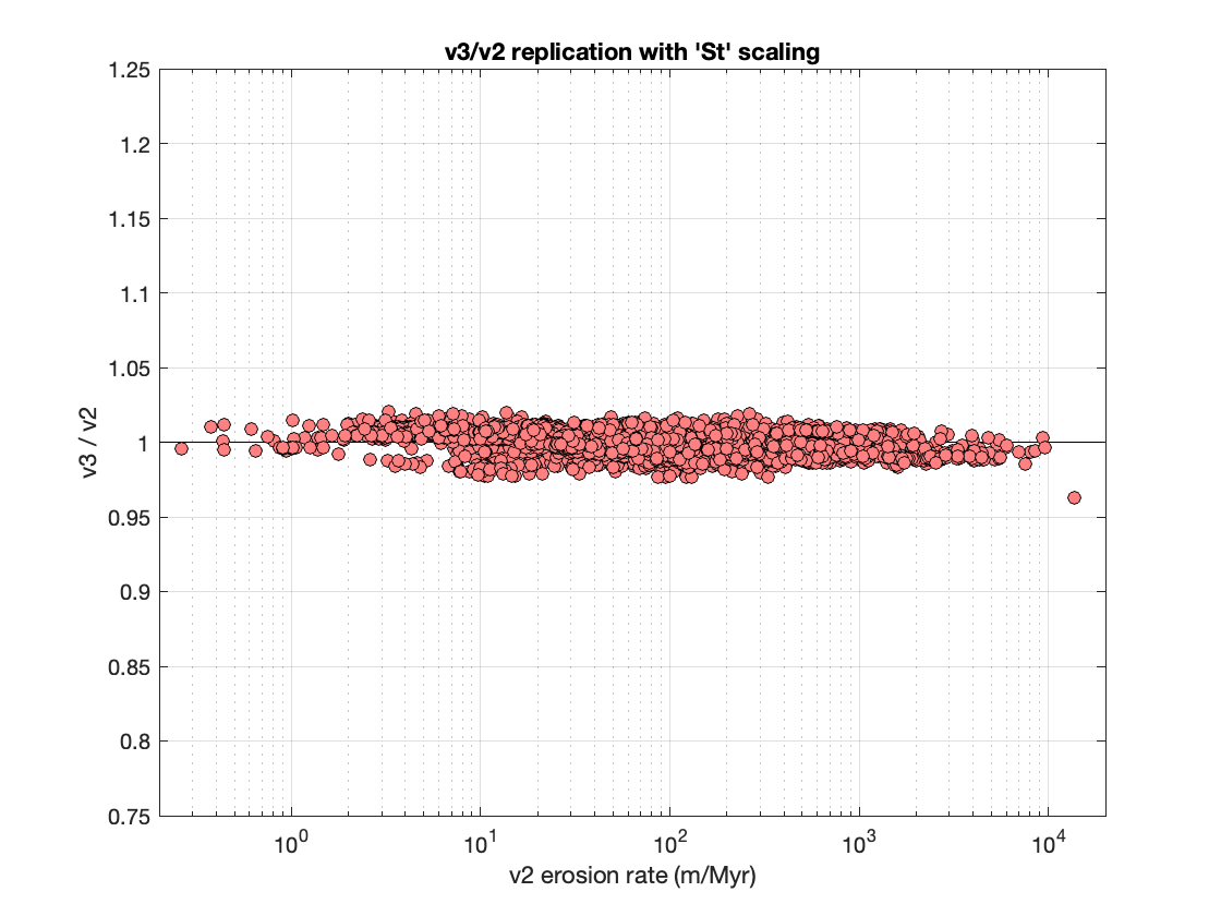
Obviously, the axes here are the erosion rate from the v2 code and the ratio of erosion rates calculated using the v3 and v2 code. Happily, they are quite similar; all the v3 results are within a couple of percent of the v2 results. Some small differences are expected and have to do with small changes between v2 and v3, including (i) a different elevation vs. air pressure conversion, which probably accounts for most of the random scatter, and (ii) different handling of muon-produced Be-10, which accounts for the small systematic decrease in the v3/v2 ratio with increasing erosion rate. But, in general, this comparison reveals no systematic problems and counts as a pass.

Task 2 is to compare the results of the v2 and v3 code for time-dependent “Lm” scaling. This is a bit more complicated. Frankly, it’s also a lot less relevant because the time-dependent scaling methods are not widely used for erosion rate applications. The issue of which scaling method to use is relatively minor by comparison with all the other assumptions that go into a steady-state erosion rate calculation, so most researchers don’t worry about it and use the non-time-dependent method. However, erosion rates calculated with time-dependent scaling have some interesting properties that are potentially useful in figuring out whether things are working as they should, so here are the results:

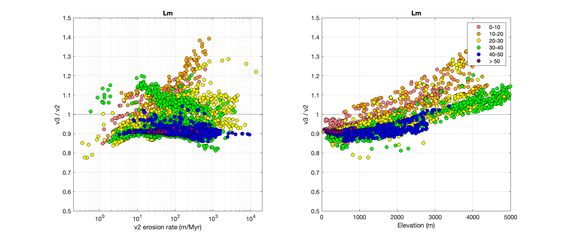
Again, the y-axis in both plots is the ratio of erosion rates calculated using the v3 and v2 implementations of Lm scaling, the x-axes are apparent erosion rate on the left and elevation on the right, and the data are color-coded by latitude, as shown in the legend. This turns out to be kind of a strange plot. At low latitude, there are some fairly large differences between the results of the v2 and v3 code, and there is a systematic difference between v3 and v2 results that varies with latitude. At high latitude, v3 results are a bit lower; at low latitude they are a bit higher with a difference that depends on elevation. These differences appear to be mostly the result of a change in how the v3 implementation of Lm scaling relates geomagnetic latitude to cutoff rigidity. This, in turn, affects how the Lal scaling polynomials, which were originally written as a function of geomagnetic latitude, map to cutoff rigidity values in paleomagnetic field reconstructions. The implementation in version 3 is supposed to be more consistent with how the cutoff rigidity maps in the field reconstructions were calculated. Another change between version 2 and 3 is that the paleomagnetic field reconstruction is different, so that also contributes to the differences and most likely accounts for a lot of the nonsystematic scatter, especially at erosion rates in the hundreds-of-meters-per-million-years range where the Holocene magnetic field reconstruction is important. The point, however, is that these differences appear to be more or less consistent with what we expect from the changes in the code — so far there is no evidence that anything is seriously wrong with version 3.

That pretty much completes the main point of this exercise, which was to establish, by comparison with version 2, that there doesn’t seem to be anything seriously wrong with version 3. This is good, because version 3 is much faster. However, having set up the whole test data set and calculation framework, there is some other interesting stuff we can do with the results.

The first interesting thing is that the calculations apply both time-dependent and non-time-dependent scaling methods to the same data set. This is a neat opportunity to see what the effect of time-dependent scaling in erosion rate calculations is. Here is the effect:

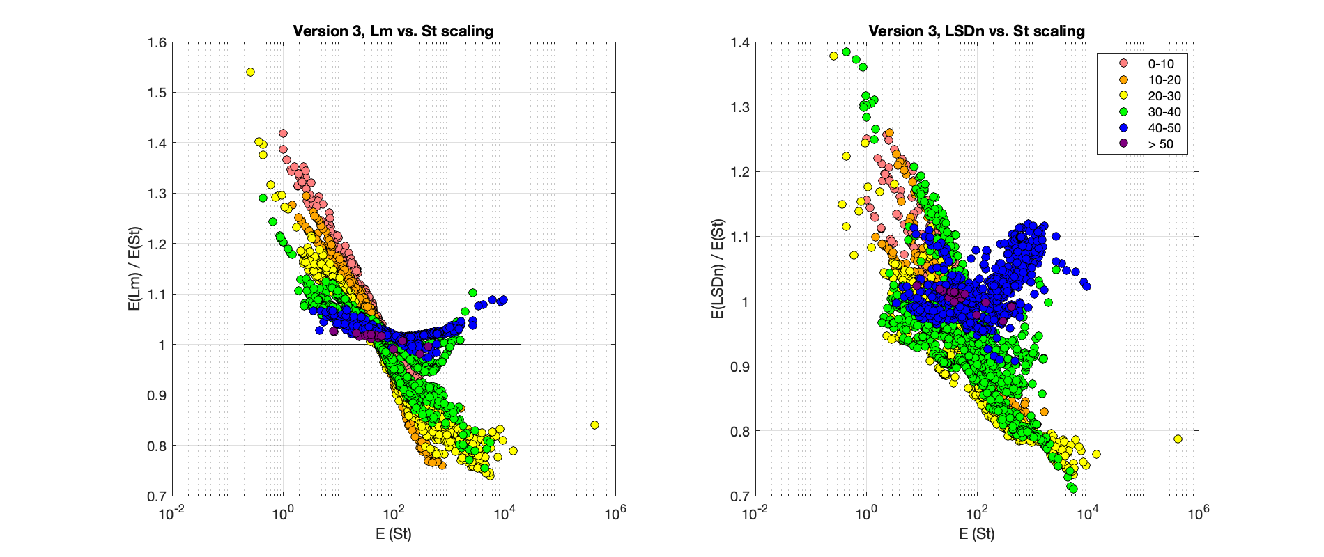
This is another complicated figure that looks like the last one, but is actually showing something different — the previous figure was comparing two different versions of Lm scaling, whereas this one is comparing the results of a time-dependent method (Lm on the left, LSDn on the right) with the non-time-dependent St scaling.

The main thing that this shows is that using a time-dependent scaling method makes a difference. Basically, the measured nuclide concentration in a sample with a higher erosion rate is integrating production over a shorter time than that in a sample with a lower erosion rate. In other words, samples with different erosion rates are sampling different parts of the paleomagnetic field record. Because the present magnetic field seems to have been anomalously strong by comparison with the last couple of million years, samples with lower erosion rates have, on average, experienced periods of lower magnetic field strength and therefore higher production rate. For samples with erosion rates around 100 m/Myr, most of the measured nuclide concentration was produced during the past 20,000 years, which also happens to be the approximate age range of most of the production rate calibration data that are used to calibrate all the scaling methods. Thus, calculated erosion rates in this range are about the same for time-dependent and non-time-dependent scaling. Samples with lower erosion rates reflect production during longer-ago periods of weaker magnetic field strength and higher production rates, so an erosion rate computed with time-dependent scaling will be higher than one computed with non-time-dependent scaling. These plots also show that this effect is most pronounced for samples at lower latitudes where magnetic field changes have a larger effect on the production rate. The final thing that is evident in these plots is the difference between Lm and LSDn scaling. The elevation dependence of the production rate is the same for both St and Lm scaling, so differences are closely correlated with latitude and erosion rate; this is evident in the minimal scatter around the central trend for each color group in the left-hand plot. On the other hand, LSDn scaling has a different production rate – elevation relationship, so the fact that the samples in each group are all at different elevations leads to a lot more scatter. But overall, the relationship is basically the same.

Although, as noted, time-dependent scaling methods mostly aren’t used for erosion rate studies, it’s worth thinking a bit about whether or not this is a potential problem. The main thing that most erosion rate studies are trying to do is look for correlations between erosion rates and something else — basin slope, relief, whatever. Thus, if you created spurious variations in calculated erosion rates by using a non-time-dependent instead of a time-dependent method, you might incorrectly attribute that variation to some characteristics of the basins. For basins that are reasonably close together, the data in the plot above shows that this isn’t likely to be a problem — the difference in scaling method is essentially just applying a monotonic stretch to the erosion rates, so it might increase the size of variations, but not create variations that weren’t there already.  However, for basins that span a wide range of location and elevation, or for global compilations, this might be something to pay attention to.

The second interesting side project we can do with this data set is to compare the results of erosion rates calculated using the version 3 calculator with the erosion rates that were calculated as part of the OCTOPUS project and are reported in the OCTOPUS database. These calculation methods are very different, and, in addition, here is where all the simplifying assumptions we made in generating the test data set become important. For the version 3 calculations, as described above, we approximated each basin by a central point and a mean elevation. Choosing a single location for the basin doesn’t make a ton of difference, but using the mean elevation is nearly always wrong, and will mostly underestimate the true average production rate in the basin, because the production rate – elevation relationship is nonlinear. Although the OCTOPUS calculations use St scaling, the approximations for muon production are different, and, most importantly, they use the much more elaborate ‘CAIRN‘ erosion rate calculation, which considers all the pixels in the basin as sediment sources with different production rates and obtains the erosion rate by numerically solving a complete forward model calculation of the nuclide concentration. In principle, this method is much better because it is much more realistic, and generally much less dumb, than approximating the basin by a single point. On the other hand, it also incorporates at least one thing — an adjustment to production rates for topographic shielding effects — that we now know to be incorrect. Of course, the point of recalculating all the OCTOPUS data with the v3 calculator code wasn’t to generate more accurate erosion rate estimates than the CAIRN estimates — it was just to take advantage of an easily available data set for benchmarking — but quite a lot of the erosion rate literature does use single-point-approximations for basin-scale erosion rate calculations, so it’s interesting to look at the differences (even though the CAIRN paper already did this, the v3 code wasn’t available at that point). Anyway, here are the differences.

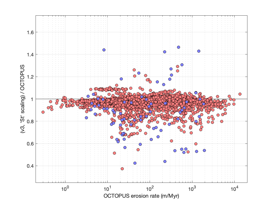
Here I have split out Be-10 (red) and Al-26 (blue), which highlights that there aren’t a whole lot of Al-26 data. Overall, this is not bad. There doesn’t appear to be any systematic offset with erosion rate, so here it is as a single histogram:

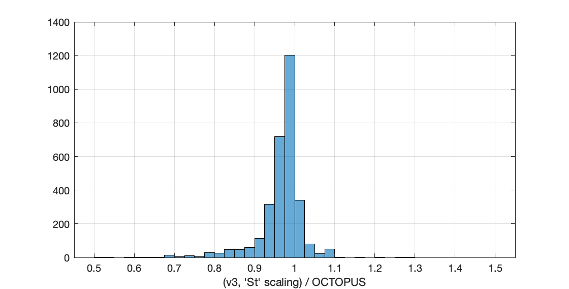
There is a small systematic offset (4% to the low side) that appears to be the result of using different muon calculations and slightly different production rate calibrations,  a decent amount of scatter (the standard deviation is 6%), and some weird outliers. We expect quite a lot of scatter because of the single-point approximation — the difference between the results of full-basin and single-point calculations will vary with basin elevation, relief, and hypsometry, which of course are different for all basins. I think we expect the scatter to be skewed to the low side in these results, because the effective elevation is nearly always higher than the mean elevation, and this effect does appear in the histogram. As regards the handful of weird outliers, I did not try to figure them out individually.

Regardless, the fact that the version 3 results are more or less in agreement with the OCTOPUS results also generally seems to indicate that nothing is seriously wrong. The version 3 code may be safe to use.

 

 

Can we switch yet?

No, not switch governments — switch exposure-age calculators. Sorry. This post is about the really excessively long transition from the not-so-recent to the most-recent version of the online exposure age and erosion rate calculators.

It is true that this subject is less important than the news of the day, which is that the entire top of the US military command structure, including the Joint Chiefs of Staff, is now in preventative quarantine. Leaving that aside for the moment, though, the background to this post, detailed here, is that various iterations of the so-called “version 2” of the online exposure age calculators were in use from the middle of 2007, shortly after the whole thing was invented in the first place, until approximately 2017. In 2017, I developed an updated “version 3” that had more features, fewer scaling methods, and was much faster. However, adoption was rather slow, most likely because (i) people like what they’re used to, and (ii) while the version 2 calculators came with an actual, Good-Housekeeping-Seal-Of-Approval peer-reviewed paper describing them, as well as ridiculously comprehensive documentation, version 3 has no paper and unimpressive documentation. The no-paper part seems to lead to difficulty in figuring out how to cite the version 3 calculators in a paper and, perhaps, a diffuse, creeping sense of doubt about whether or not they are really legit or authorized. Frankly, the quite-poor-by-comparison-to-version-2 documentation doesn’t help. This could be improved.

Regardless, the version 3 calculators are better. They are faster, replace scaling methods known to be inaccurate with a more up-to-date one that is known to be more accurate, and compute ages for many different nuclide/mineral systems instead of just Be-10 and Al-26. They are much better. The point of this post is to determine whether the user community is, in fact, figuring this out and switching.

The following shows two things. In the top panel, total manual usage of the online exposure age calculators during the past 5 years. “Manual” in this case means that users actually cut-and-pasted data into the online entry forms. The majority of the total calculation load on the version 3 online calculators is not from manual entry, but instead from the automated, dynamic calculations associated with serving web pages for the ICE-D databases, and these are not included here. Manual usage of the online exposure age calculators has been remarkably stable over the past several years around an average of about 8500 exposure-age requests monthly.

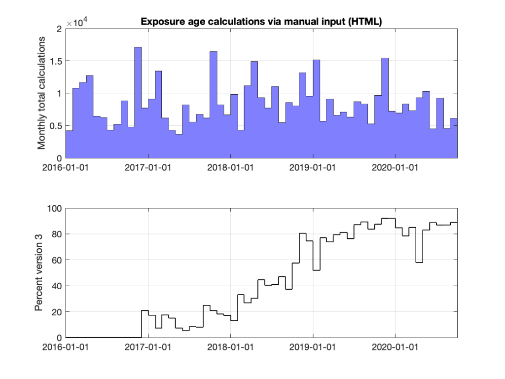
The bottom panel shows the fraction of those requests that use version 3 rather than version 2. It took almost three years and the switchover was remarkably gradual, but at this point it appears that nearly everyone has switched. As version 3 of the exposure age calculators has now been fairly well debugged and is pretty much known to work, it is probably time to take version 2 off the front page and move it to the archives. While it certainly deserves some wall space next to a hunk of Libyan Desert Glass in any future museum of exposure dating, I think we are done with it.

That’s just the exposure-age calculations, though. The online erosion rate calculators get about 15% of the usage of the exposure age calculators, so weren’t a priority in developing version 3, and this part of version 3 was somewhat delayed. As with the exposure-age calculations, however, the erosion-rate parts of version 3 are generally better and very, very much faster than the equivalent bits of version 2. On the other hand, they are even less well documented than the exposure-age calculations and the details are a bit murky. Total usage of the online erosion rate calculators, as with exposure-dating, has been a bit patchy but fairly stable around an average of 1500 calculations/month. Again, this doesn’t include automated use in the back end of the ICE-D X OCTOPUS web server, but that is fairly minor.

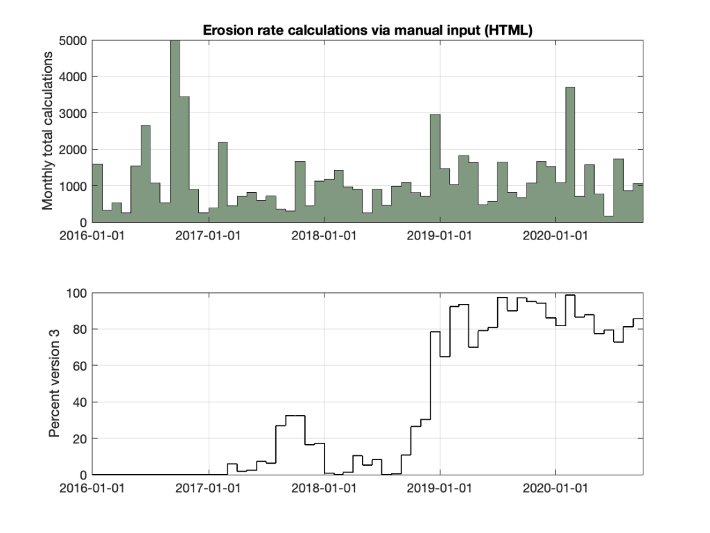
Regardless, most users of the erosion rate calculators now seem to have switched as well. The pattern is interesting: there appears to have been a trial period in late 2017 that resulted in users recoiling in horror and going back to version 2, followed by a rapid, abrupt, and globally synchronous rediscovery near the end of 2018. This is odd, but the result is the same as for exposure-age calculation — the new version now gets about 90% of the traffic. However, the version 3 erosion rate code has not been as well tested as the exposure-age code, and there are still a couple of known bugs having to do with integrating muon production for extremely fast erosion rates in the range of km/Myr. Thus, we are probably not quite ready to take version 2 off the front page for erosion rates.

Summary: nearly everyone has gotten over their doubts about the documentation and switched. Good.

Ne-21 production rate calibration demystified. Or not.

Neon-21 is now ‘trending’ on this website, because this is the second post about it this year. The purpose of this one is to try to unscramble the tedious and obscure subject of production rate calibration for cosmogenic neon-21 in quartz. Eventually, at the end, it describes an update to the part of the online exposure age calculator dealing with Ne-21, which doesn’t fix everything, but is a legitimate conceptual improvement and results in only small differences between Ne-21 exposure ages calculated before the update (i.e., yesterday) and after (today).

Even though Ne-21 production in quartz considered by itself  is nearly all just by neutron spallation and isn’t any more complicated than production of Be-10, Al-26, or He-3, it is a messy nuclide-mineral system to calibrate because measurement of cosmogenic Ne-21 has a terrible signal-to-noise ratio compared to these other nuclides.

The reason for this is simply that there is a lot of non-cosmogenic Ne-21 out there, both present as a trace isotope in all sources of natural neon (like the atmosphere) and also produced in minerals indirectly from decay of natural uranium and thorium. It is easily possible to identify and correct for atmospheric neon based on its isotope ratio, but even after doing this there is nearly always some extra non-cosmogenic Ne-21 in quartz. Ne-21 is not radioactive, so the only way to get rid of it is to heat the quartz up to high temperature. Most quartz in typical rocks at the Earth’s surface has been below the neon retention temperature for tens or hundreds of millions of years, and contains quite a lot of non-cosmogenic (“nucleogenic”) Ne-21 produced from U and Th decay, so can contain nucleogenic Ne-21 equivalent to tens or hundreds of thousands of years of surface exposure. Suppose you go to a site where the production rate of cosmogenic Ne-21 is about 20 atoms/g/yr, pick up a rock, and observe 2 Matoms/g of Ne-21 in the quartz. This rock could really have a 100,000 year exposure age, or it could have arrived at the surface yesterday with a lot of nucleogenic Ne-21. Hard to tell.

This property of Ne-21 is a serious problem for production rate calibration because of how calibration normally works. Normally, we find a rock surface that we already know the exposure age of, usually by radiocarbon dating of related deposits. We measure the amount of, say, cosmogenic beryllium-10, divide the number of atoms per gram of Be-10 by the age, and obtain the Be-10 production rate in atoms per gram per year. This is quite straightforward if you can find rock surfaces that have been exposed for a known amount of time and also have not been disturbed or eroded since they were emplaced. Unfortunately, you can generally only do this for sites that are relatively young. Most good production rate calibration sites have exposure ages less than about 20,000 years, and the reason for this is that rock surfaces in most environments simply do not survive in pristine condition for a lot longer than this. Older surfaces get eroded, weathered, flaked, spalled, covered, uncovered, and generally messed up, which makes them hard to use for production rate calibration. If the surfaces that are good for production rate calibration have short exposure durations, they also have low concentrations of cosmogenic Ne-21. For nearly all production rate calibration sites that we have used for Be-10 and Al-26 calibration, concentrations of cosmogenic Ne-21 in quartz are lower than concentrations of non-cosmogenic Ne-21. Even if you measure the total amount of Ne-21 very precisely, and also you could estimate the amount of non-cosmogenic Ne-21 very precisely (which is usually impossible for a variety of reasons), estimating cosmogenic Ne-21 would still involve subtracting one big number from another big number to yield a small number. This results in a small number with a big uncertainty.

So, a surface that is good for direct production rate calibration has to be young enough that it is still pristine, but if this is true it is also too young to make a decent measurement of the cosmogenic Ne-21 concentration. This is extremely inconvenient. Most attempts to estimate the Ne-21 production rate, therefore, have had to use much more complicated strategies, mostly based on the idea of finding surfaces that have very high concentrations of cosmogenic Ne-21 so any correction for nucleogenic Ne-21 is negligible, but also have some kind of back story that enables you to make a believable argument about what the long-term exposure history has been, so you can assume an exposure history and back-calculate the production rate. One example, which I will focus on here because it is more polite to highlight the weaknesses of my own work than of others’, is a 2009 paper about rock surfaces in the Antarctic Dry Valleys. This involves a handful of samples from slowly eroding rock surfaces that are believed to have been ice-free and slowly weathering for millions of years, and also have Be-10 and Al-26 concentrations that are consistent with production-decay-erosion steady state. In other words, their Be-10 and Al-26 concentrations lie on the steady erosion line in a 2-nuclide diagram:

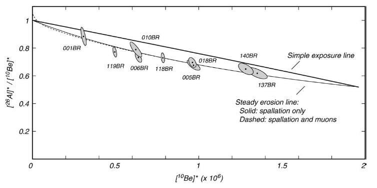
So, we assume that these samples have also reached production-erosion equilibrium for Ne-21. Then if the cosmogenic Ne-21 concentration is N21, the production rate is P21, the erosion rate inferred from the Be-10 and Al-26 concentrations is E, and we ignore muon production for the moment, P21 = N21*E/L, where L is the attenuation depth constant for spallogenic production (Lambda in most places). Basically, we are asking, OK, what Ne-21 production rate is needed to make it so that these data are also on the steady erosion line in Al-26/Ne-21 and Be-10/Ne-21 diagrams?

The advantage of this approach is that these surfaces are eroding very slowly, so cosmogenic Ne-21 concentrations are about two orders of magnitude higher than nucleogenic concentrations. It is easy to accurately measure the cosmogenic Ne-21 concentration. The disadvantage is that the back story involves a lot of assumptions. As noted, we have  to assume that the surfaces really are at erosional steady state. That might be true, but we also rely on accurately knowing the Al-26 and Be-10 production rates, so that we get the right erosion rate to plug into this formula. To some extent the dependence on the Be-10 production rate can be mitigated if you compute a ratio of Ne-21 to Be-10 production rates, and this paper eventually concluded that the Ne-21/Be-10 production ratio is 4.08. This more or less agrees with the conclusions of four other papers that used similarly devious and complex strategies, particularly including a very creative one by Florian Kober and Vasily Alfimov, as well as an additional paper describing an early attempt to determine the Ne-21 production rate directly from a young surface by Samuel Niedermann. Since approximately 2009, therefore, folks have mostly assumed that the Ne-21/Be-10 production ratio is close to 4, and computed Ne-21 production rates by applying this ratio to their best estimate of the Be-10 production rate.

This is what the Ne-21 production rate calibration in version 3 of the online exposure age calculators, at least as of last week, is based on. I think that’s the only online exposure age calculator that accepts Ne-21 input at all. This assumption mostly seems to work pretty well, but to get to the main point of this post, if you look at this carefully, it is not really clear that it should work at all, or if it is a good idea. For example, here are some problems.

The main problem is that the production ratio estimate from the Dry Valleys data described above is based on an impressive number of assumptions that were fine at the time, but are now known to be obsolete or incorrect. One: the erosion rates calculated from the Be-10 and Al-26 concentrations are based on obsolete production rate calibration data that have since been discovered to be inaccurate. Basically, the Be-10/Al-26 production rates were too high, which means the estimates of the erosion rates are also too high. Two: these calculations also used a Be-10 half-life that we now know is wrong. Because the erosion rates are so low, the half-life update affects the erosion rate estimate. Three: AMS standardization of Be-10 measurements had not fully been sorted out when that paper was written, which is related to the production rate and half-life revisions. Four: that paper assumes that the quartz samples had zero nucleogenic Ne-21. Later investigation has shown that they have a fairly large amount. Five: that paper concluded that muon production of Ne-21 was fairly high. It is now known from other data to be lower. Six: recent interlaboratory comparisons show that the Ne-21 concentrations in that paper need to be adusted.

This is a huge list of things that we know are wrong and need to be updated.

Disappointingly, another recent paper (also by me) addressed items (4-6) above and concluded that they had a negligible effect on the estimate of the Ne-21/Be-10 production ratio. However, it didn’t address items (1-3), which is kind of misleading, so this conclusion might be right but possibly shouldn’t have been included in the paper.

And then there is one more thing. The ‘LSDn’ production rate scaling method of Lifton and Sato (various references), which is now in common use and believed to be the most accurate available, predicts that the Ne-21/Be-10 production ratio should be variable with elevation, and this was not taken into account at all in the 2009-2011 studies. And, finally, adding insult to injury, the 2014 implementation of the LSDn scaling method did not include any estimates of the cross-sections for Ne-21 production reactions, so the online exposure age calculator has been using a generic neutron flux scaling, which predicts a ratio-elevation relationship that is not even the correct one.

So, this is about ten reasons that the currently accepted production rate calibration that is in the online exposure age calculators for Ne-21 is probably wrong. On the other hand, the other papers that all basically agree on the 21/10 production ratio are subject to a different set of obsolete inputs and assumptions, and the fact that they all basically agree may well indicate that the various inaccuracies all cancel each other out. However, it seems like a bad idea to rely on this sort of magical thinking. So the current overall credibility of the Ne-21 production rate calibration that we have mostly been using is not ideal.

Fortunately, and in sharp contrast with the arc of American history at this precise moment, there is hope. Just as we were faced with the unpleasant and possibly impossible task of trying to recalculate all the old estimates of the 21/10 production ratio with new input parameters, a new paper by Cassie Fenton and others has saved us from despair. Almost. I’ll get to the “almost” part at the end.

Here’s how. Remember the root problem with Ne-21 production rate calibration is that we can’t do a direct calibration on surfaces of known age if all we have are young surfaces with high concentrations of nucleogenic Ne-21. So, instead of doing all this fancy stuff with elaborate back stories and steady-erosion assumptions, wouldn’t it be better to just find an old but pristine rock surface that doesn’t have any nucleogenic Ne-21 in the quartz? It is hard to argue with that reasoning. The surface that Cassie and colleagues have located is a quartz-bearing basaltic lava flow in Arizona with an unprintable name having the abbreviation “SP.” When you add some other words like “Cosmogenic” and, maybe, “Intercalibration” and “Experiment” – I am not sure – you get a project called “SPICE,” which should not be confused with either the Spice Girls or the SPICE core. But the point is that they have located a 72,000-year-old quartz-bearing lava flow in the middle of a desert where erosion and surface disturbance rates are very low. And because the amount of nucleogenic Ne-21 scales with the cooling age of the rock, if you want the minimum possible amount of non-cosmogenic Ne-21, you want a rock whose cooling age is no older than the exposure age. Like a lava flow. So we have a site that is a lot older than most calibration sites and has a lot less nucleogenic Ne-21 than most other rocks. Perfect.

This is important because it means we might not have to unscramble the mess of old production ratio estimates from ten years ago. We can forget about them and move on to a better plan. This implies that from the online exposure age calculator perspective, we should do the following:

1. Fix the LSDn scaling code to use specific reaction cross sections for Si –> Ne-21. Also fix it to use up-to-date muon-related parameters from here.
2. Calibrate the various production rate scaling methods using the SPICE data.
3. Figure out if the results agree with what we were using before. Have we been doing it wrong?

We can obtain reaction cross-sections from a 2015 revision of the LSDn scaling code provided by Nat Lifton, that originate with estimates by Bob Reedy described here.  Here is what they look like:

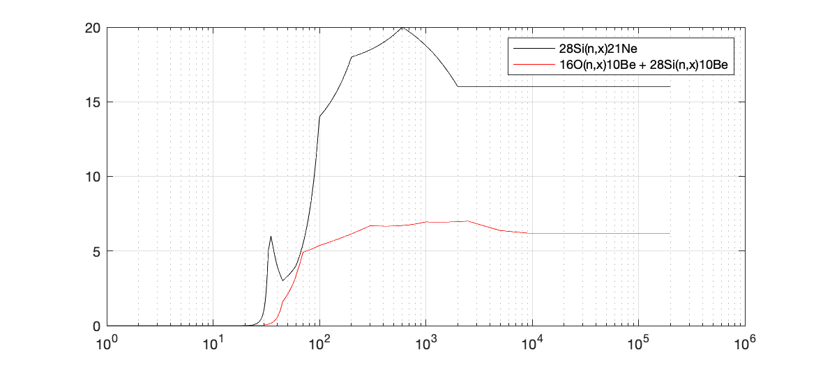This shows the energy dependence of the main production reactions for Ne-21 and Be-10, with the X-axis in MeV. The threshold energy and peak cross-section energy for Ne-21 production is a little bit higher than for Be-10, so the Ne-21/Be-10 production ratio should go up a little bit as elevation increases. This is actually the opposite of what has been in the online exposure age calculator until now: so far, the Ne-21 scaling has just used a total-neutron-flux scaling (e.g., the ‘Sf’ method in CRONUSCalc), which has no threshold energy, so will predict a higher 21/10 ratio at low elevation.

Having fixed that, we can now take the SPICE Ne-21 data, which are here, and paste them into the production rate calibration input page here (note that this posting is slightly asynchronous with the server update, so this may not look exactly like this until such time as I update the web servers to use the new scaling code). This is the result:

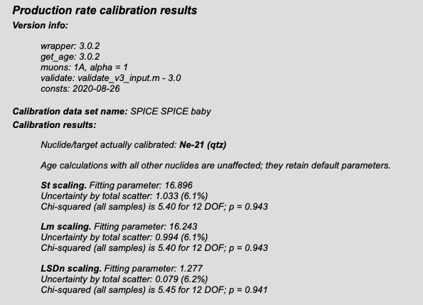
Now, compare this with what we were doing before, which was computing the Be-10 production rate and multiplying by 4. Start with ‘St’ and ‘Lm’ scaling. For these scaling methods, the fitting parameter is a dimensional spallogenic production rate (atoms/g/yr) at some reference condition. If we were to take the existing default calibrated reference production rates for Be-10 for St and Lm scaling (4.09 and 4.21 atoms/g/yr, which derive from the CRONUS-Earth ‘primary’ calibration data set here) and apply the 21/10 production ratio of about 4 that is expected from the 2009 studies, we would get 16.36 and 16.84, which are within 3-4% of the results of calibrating with the SPICE data. So that’s good. The other way to say that is that if we calibrate Ne-21 using SPICE data and Be-10 using the existing default calibration, we predict Ne-21/Be-10 production ratios of (16.896/4.09 = 4.13) and (16.243/4.21 = 3.86) for ‘St’ and ‘Lm’ scaling, which are both within 3% of the previously accepted value of 4, or basically the same given the expected precision of the various measurements. Of course this only includes spallogenic production, but both nuclides have minimal muon production so that has a negligible effect on the ratio. Even though our best estimate of the reference Be-10 production rate now is very different from the 2009 estimate — it is about 10-15% lower — these results are indistinguishable from what we thought the ratio should be at the time. So this result (which, by the way, just duplicates a conclusion that Cassie already came to in the SPICE paper) is good. We were not totally wrong before.

One interesting aspect of this result (which is also thoroughly discussed in the SPICE paper, although with slightly different conclusions) is that the apparent production ratios for the two scaling methods are different. This is unexpected because the ratio primarily results from the mineral chemistry and reaction cross-sections, so the true ratio should be close to independent of the scaling method.  On the other hand, the way the calculation is done is expected to lead to a difference here because the SPICE site is much older than the calibration sites used to estimate the Be-10 production rate, so the two calibration data sets are averaging over different time periods. Because most of the sites involved are at low enough latitude that magnetic field variations have an effect on production rates, the older site is sampling a period of lower average magnetic field strength, and therefore higher production rates, than the younger sites. The ‘Lm’ scaling method accounts for this, and the non-time-dependent ‘St’ method doesn’t. This means that St scaling with this particular combination of sites should overestimate the 21/10 production ratio by a few percent.

For LSDn scaling, the calibrated parameter is a nondimensional correction factor, not a reference production rate, and in addition the production ratio is predicted to vary with elevation, so we need to compute both Be-10 and Ne-21 production rates for a range of elevations instead of just dividing the fitted reference production rates. After calibrating Ne-21 production with the SPICE data set and leaving the Be-10 production rate calibration as the default, here is the predicted 21/10 production ratio for LSDn scaling as a function of elevation for polar latitudes (like Antarctica, where we care about this because there are a lot of Ne-21 data):

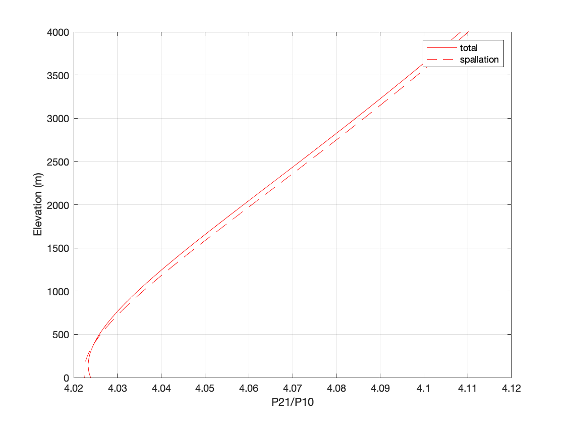Basically, it is exactly what we expected it to be based on the complex and sketchy indirect calibration scheme from 2009: at the elevation of the Dry Valleys (about 1500 m) it predicts P21/P10 = 4.05. This figure also shows what I said above, that the ratio is basically the same whether or not you ignore muons. Again, this seems good. Either we got it right the first time, or we made so many offsetting errors that we still got it right by accident. It’s a few percent higher than what we get for the also-paleomagnetically-corrected Lm scaling, but this is not necessarily significant because LSDn scaling treats each production reaction separately, whereas St and Lm treat them all the same, so the two estimates are not really comparable.

So, this seems like a complete solution for the online exposure age calculator. Disregard the messy and in-need-of-revision attempts to measure the production ratio from ten years ago. Update the various background parameters. Calibrate the Ne-21 production rate directly from the SPICE data. Done.

 

 

OK, careful readers will immediately notice that the previous paragraph ended in “Done,” but this already quite tedious posting hasn’t actually ended. This is because there is a small problem with this reasoning. Here is the problem. The SPICE calibration study didn’t just measure Ne-21 in the quartz from the SP flow…it also measured Be-10. Thus, no matter what the scaling method is and regardless of whether or not we have messed up anything to do with scaling and production rate calibration, the measured ratio of Ne-21 and Be-10 concentrations should be equal to the ratio of the production rates (or almost equal…a small correction for radioactive decay of Be-10 is needed). The production ratio computed from the measured concentrations in this study is…4.35 +/- 0.23. Which is 5-10% larger than we think it should be from both the old calibration studies and the paragraphs above that compare Ne-21 and Be-10 production rates calibrated using separate data sets. Theoretically, measuring both nuclides in the same quartz at the same site should be a better estimate of the production ratio than comparing production rates calibrated from different data sets, so this is weird.

On closer examination, what is happening here is that the Be-10 concentrations measured here are lower than we expect from other production rate calibrations. In other words, as noted at length in the SPICE paper, production rates calibrated using the SPICE Be-10 data alone are 5-10% lower than those calibrated using the rest of the global data set, depending on which scaling method is used. This is not just an artifact of the fact that most of the global calibration data are much younger, because it’s true for both paleomagnetically corrected and uncorrected scaling methods. And, in addition, Be-10 production rates that are as low as predicted by the SPICE data are inconsistent with many Be-10 data from Antarctica that are from surfaces with near-zero erosion rates and are close to production-decay saturation. If production rates were as low as predicted by the SPICE Be-10 data, predicted saturation concentrations would be 10% lower than the measured concentrations in these samples, which is impossible. To see an example of this calculation, take the Be-10 calibration data from here, put it in the production rate calibration page here, and then use the result to calculate Be-10 exposure ages for samples from this site.

So, the reason the apparent P21/P10 ratio at this site is a little anomalous is actually not because of the Ne-21 data, but because the Be-10 data are anomalous with respect to the rest of the world. There could be a couple of reasons for this.

Option 1 is the elaborate one. In this option, we solve the mismatch between these Be-10 data and others by arguing that there has been unrecognized erosion at the site. 18 cm of erosion in 72 ka would make the Be-10 data agree with other calibration data. But then we have too much Ne-21, so we need to solve that by arguing that 5-10% of the Ne-21 is actually nucleogenic and not cosmogenic. This is rather unlikely, as nucleogenic production of 10% of the observed excess Ne-21 in 72 ka would require something like 50 ppm U and Th in the quartz, which is about two orders of magnitude more than typically observed. Theoretically one could appeal to trapped magmatic neon with some strange isotope composition, but overall that is not a very good explanation.

Option 2 is that the Ar-Ar age is inaccurate and the flow is really a bit younger. However, quite a lot of work has gone into the Ar-Ar dating and there is no reason to suspect this. This option also requires that 10% of the Ne-21 is noncosmogenic, as above.

Option 3 is the simple one and involves concluding that the Be-10 measurements are systematically a little too low, and the Ar-Ar age and the Ne-21 measurements are correct. The argument against this option is that there is no reason to think that any measurement errors were made in this study. The Be-10 measurements should be totally fine. On the other hand, a ~10% difference is not too far out of the range of normal measurement scatter. So this would tend to indicate that we should calibrate the Be-10 production rate using a large data set from many sites (of which the SPICE data are a moderate, although not extreme, outlier), and the Ne-21 production rate using the SPICE data (because there are no other equivalent sites, so they are the entire global data set for Ne-21). This is probably the least unsatisfying option.

Summary: the online exposure age calculator is now updated to use this approach going forward, even though this is still a bit unsatisying, because the concentration ratio measured at any one site should agree with the production ratio estimated from large calibration data sets, and the fact that it doesn’t means that we are missing something. Even though this is not perfectly satisfying, remember, the screwup we are arguing about now is only a 5% effect. That’s pretty good. So, we will be happy that this approach agrees with all other estimates of the P21/P10 ratio, and we will temporarily ignore the fact that it doesn’t quite agree with the measured concentration ratios. Because this site turns out to be so transformatively useful for Ne-21 production rate calibration, though, it would probably also be a good idea to take some steps to try to unscramble this, including (i) sending some SPICE quartz to additional labs to deal with the possibility of measurement error for both Be-10 and Ne-21, (ii) maybe replicating the Ar-Ar age a couple more times, and (iii) looking for a shielded sample of the SP flow to see if there is any noncosmogenic Ne-21. Unfortunately, a quick Google Maps search did not disclose any road cuts or borrow pits in the flow, so the shielded sample might be tough.